Emergent behaviors of Lohe Hermitian sphere particles under time-delayed interactions

  • Received: 01 January 2021 Revised: 01 April 2021 Published: 20 May 2021
  • Primary: 82C10, 82C22, 35Q40

  • We study emergent behaviors of the Lohe Hermitian sphere(LHS) model with a time-delay for a homogeneous and heterogeneous ensemble. The LHS model is a complex counterpart of the Lohe sphere(LS) aggregation model on the unit sphere in Euclidean space, and it describes the aggregation of particles on the unit Hermitian sphere in Cd with d2. Recently it has been introduced by two authors of this work as a special case of the Lohe tensor model. When the coupling gain pair satisfies a specific linear relation, namely the Stuart-Landau(SL) coupling gain pair, it can be embedded into the LS model on R2d. In this work, we show that if the coupling gain pair is close to the SL coupling pair case, the dynamics of the LHS model exhibits an emergent aggregate phenomenon via the interplay between time-delayed interactions and nonlinear coupling between states. For this, we present several frameworks for complete aggregation and practical aggregation in terms of initial data and system parameters using the Lyapunov functional approach.

    Citation: Seung-Yeal Ha, Gyuyoung Hwang, Hansol Park. Emergent behaviors of Lohe Hermitian sphere particles under time-delayed interactions[J]. Networks and Heterogeneous Media, 2021, 16(3): 459-492. doi: 10.3934/nhm.2021013

    Related Papers:

    [1] Seung-Yeal Ha, Gyuyoung Hwang, Hansol Park . Emergent behaviors of Lohe Hermitian sphere particles under time-delayed interactions. Networks and Heterogeneous Media, 2021, 16(3): 459-492. doi: 10.3934/nhm.2021013
    [2] Young-Pil Choi, Cristina Pignotti . Emergent behavior of Cucker-Smale model with normalized weights and distributed time delays. Networks and Heterogeneous Media, 2019, 14(4): 789-804. doi: 10.3934/nhm.2019032
    [3] Tingting Zhu . Synchronization of the generalized Kuramoto model with time delay and frustration. Networks and Heterogeneous Media, 2023, 18(4): 1772-1798. doi: 10.3934/nhm.2023077
    [4] Jérôme Fehrenbach, Jacek Narski, Jiale Hua, Samuel Lemercier, Asja Jelić, Cécile Appert-Rolland, Stéphane Donikian, Julien Pettré, Pierre Degond . Time-delayed follow-the-leader model for pedestrians walking in line. Networks and Heterogeneous Media, 2015, 10(3): 579-608. doi: 10.3934/nhm.2015.10.579
    [5] Marina Dolfin, Mirosław Lachowicz . Modeling opinion dynamics: How the network enhances consensus. Networks and Heterogeneous Media, 2015, 10(4): 877-896. doi: 10.3934/nhm.2015.10.877
    [6] Michael Helmers, Barbara Niethammer, Xiaofeng Ren . Evolution in off-critical diblock copolymer melts. Networks and Heterogeneous Media, 2008, 3(3): 615-632. doi: 10.3934/nhm.2008.3.615
    [7] Maksym Berezhnyi, Evgen Khruslov . Non-standard dynamics of elastic composites. Networks and Heterogeneous Media, 2011, 6(1): 89-109. doi: 10.3934/nhm.2011.6.89
    [8] Hyeong-Ohk Bae, Seung Yeon Cho, Jane Yoo, Seok-Bae Yun . Effect of time delay on flocking dynamics. Networks and Heterogeneous Media, 2022, 17(5): 803-825. doi: 10.3934/nhm.2022027
    [9] Paolo Antonelli, Seung-Yeal Ha, Dohyun Kim, Pierangelo Marcati . The Wigner-Lohe model for quantum synchronization and its emergent dynamics. Networks and Heterogeneous Media, 2017, 12(3): 403-416. doi: 10.3934/nhm.2017018
    [10] Junyuan Lin, Timothy A. Lucas . A particle swarm optimization model of emergency airplane evacuations with emotion. Networks and Heterogeneous Media, 2015, 10(3): 631-646. doi: 10.3934/nhm.2015.10.631
  • We study emergent behaviors of the Lohe Hermitian sphere(LHS) model with a time-delay for a homogeneous and heterogeneous ensemble. The LHS model is a complex counterpart of the Lohe sphere(LS) aggregation model on the unit sphere in Euclidean space, and it describes the aggregation of particles on the unit Hermitian sphere in Cd with d2. Recently it has been introduced by two authors of this work as a special case of the Lohe tensor model. When the coupling gain pair satisfies a specific linear relation, namely the Stuart-Landau(SL) coupling gain pair, it can be embedded into the LS model on R2d. In this work, we show that if the coupling gain pair is close to the SL coupling pair case, the dynamics of the LHS model exhibits an emergent aggregate phenomenon via the interplay between time-delayed interactions and nonlinear coupling between states. For this, we present several frameworks for complete aggregation and practical aggregation in terms of initial data and system parameters using the Lyapunov functional approach.


    Emergent dynamics of a many-body system is ubiquitous in classical and quantum systems, e.g., aggregation of bacteria [38, 39], flocking of birds [2], schooling of fish, synchronization of fireflies and neurons [7, 34, 41, 42] and hand clapping of people in a concert hall, etc. For surveys and books, we refer to [1, 2, 4, 16, 19, 35, 36, 40, 42]. In this paper, we continue studies begun in [8, 24] on the emergent dynamics of the LHS model. The LHS model corresponds to the complex counterpart of the Lohe sphere(LS) model which has been extensively studied in previous literature [11, 26, 32, 33, 37, 43]. The LHS model is the first-order aggregation model describing continuous-time dynamics of particle's position on the Hermitian unit sphere HSd1:={z=([z]1,,[z]d)Cd:z:=dα=1|[z]α|2=1} with d1. Here we denote the α-th component of the complex vector zCd as [z]α which is consistent with earlier notation in [23]. As a warmup for our discussion, we briefly introduce the LHS model with time-delayed interactions.

    Let zj=([zj]1,,[zj]d)Cd be a position of the j-th Hermitian Lohe particle on the Hermitian unit sphere, and interaction weight between the j-th and k-th particle is denoted by the real value ajkR. Then, the temporal dynamics of zj is governed by the Cauchy problem to the LHS model with a uniform time-delay τ>0:

    {˙zj=Ωjzj+κ0Nkjajk(zj,zjzτkzτk,zjzj)+κ1Nkjajk(zj,zτkzτk,zj)zj,t>0,zj(t)=φj(t)HSd1,τt0,jN:={1,,N}, (1)

    where zτk(t):=zk(tτ), φj=φj(t) is a bounded continuous function of t, Ωj is a d×d skew-Hermitian matrix and (aik)RN×N is a symmetric matrix whose components are all positive. Before we continue further, we introduce

    w,z:=dα=1[ˉw]α[z]α,z:=z,z,ˉw=(¯[w]1,,¯[w]d).

    A global well-posedness of system (1) can be done by combining a local well-posedness from the standard Cauchy-Lipschitz theory in [25, 28] and a priori uniform bound in Lemma 2.1. In the absence of time-delay with τ=0, emergent dynamics of the LHS model was investigated in [8, 24] in which several sufficient frameworks were proposed for complete and practical aggregations. In this paper, we are interested in the following simple question:

    "Under what conditions on system parameters κ0,κ1,τ, network topology (aij) and initial data set {φj}, can we verify the emergence of collective behaviors of the LHS with time-delay?"

    This question has been already addressed for other low-rank aggregation models (rank-1: vectors or rank-2: matrices), to name a few, the Lohe sphere model [9, 10], the Lohe matrix model [18]. Throughout the paper, we set

    Z:=(z1,,zN),D(Z):=max1i,jNzizj.

    Next, we recall several induced concepts on the emergent dynamics of tensors [23, 24] in the following definition.

    Definition 1.1. Let {zi} be a global solution to (1).

    1. Complete aggregation occurs asymptotically if the ensemble diameter D(Z) tends to zero asymptotically:

    limtD(Z(t))=0.

    2. Practical aggregation (with respect to time-delay) occurs asymptotically if the ensemble diameter D(Z) satisfies

    limτ0+lim suptD(Z(t))=0.

    3. Practical aggregation (with respect to time-delay and coupling strength κ0) occurs asymptotically if the ensemble diameter D(Z) satisfies

    limκ0limτ0+lim suptD(Z(t))=0.

    Then, it is easy to see that complete aggregation implies practical aggregation. In the absence of time-delay τ=0, emergent dynamics for (1) has been extensively studied in [24] (see Section 2.3). Thus, main point of this paper is to analyze the effect of time-delayed interactions in the emergent dynamics of (1). For notational simplicity, we set

    maxi,j:=max1i,jN,mini,j:=min1i,jN,kj:=Nk,j=1kj.

    The main results of this paper are threefold. First, we consider the following setting:

    aik1,Ωj=0,i,kN.

    In this case, system (1) becomes

    {˙zj=κ0Nkj(zj,zjzτkzτk,zjzj)+κ1Nkj(zj,zτkzτk,zj)zj,t>0,zj(t)=φj(t)HSd1,τt0. (2)

    When the coupling gain pair (κ0,κ1) is close to the SL coupling gain pair, i.e.,

    ˜κ:=κ02+κ1,|˜κ|1,

    system (2) can be rewritten as follows (see Section 3):

    {˙zj=κ0Nkj(zj,zjzτkRe(zτk,zj)zj)+˜κNkj(zj,zτkzτk,zj)zj,t>0,zj(t)=φj(t)HSd1,τt0. (3)

    Our first set of results is concerned with the complete aggregation of (3) (see Theorem 3.1 and Theorem 3.6). We assume that system parameters and initial data satisfy

    κ0>0,|˜κ|κ0,τ1,N3,supτt0D(Z(t))1.

    For the complete aggregation, we introduce a Lyapunov functional:

    Eij(t):=zi(t)zj(t)2+γttτzi(s)zj(s)2ds,

    where γ is a constant to be determined later. Then, in Section 3, we show that Eij(t) satisfies the energy estimate (see Section 3.2.2):

    Eij(t)+βt0zi(s)zj(s)2dsEij(0),t>0,

    for some positive constant β. By Barbalat's lemma [3], the above estimate leads to the complete aggregation (see Theorem 3.6):

    limtzi(t)zj(t)=0.

    Now, our second set of result deals with the practical aggregation with respect to time-delay (Theorem 4.1). We assume that system parameters and initial data satisfy

    aij=1,Ωj=0,2|κ1|<κ0,maxi,j(1z0i,z0j)<12|κ1|κ0.

    Then, the practical aggregation (with respect to the size of time-delay) emerges:

    limτ0lim suptmaxi,j(1zi(t),zj(t))=0.

    Our final set of result is concerned with the practical aggregation with respect to both time-delay and free flow matrix Ωj (Theorem 4.7). For system (1), we assume that system parameters satisfy

    Nk=1|aikajk|Nk=1(aik+ajk)<12andmaxi,j|1z0i,z0j|<12Nk=1|aikajk|Nk=1(aik+ajk). (4)

    Note that for any unit complex vectors z0i and z0j, we have

    |1z0i,z0j|12z0iz0j2,

    Thus, relations (4) implies restriction on initial diameter and network structure:

    D(Z0):=maxi,jN|z0jz0i|24Nk=1|aikajk|Nk=1(aik+ajk). (5)

    For all-to-all network structure with aij=1, the R.H.S. of (5) becomes

    D(Z0)2,

    which is true for any initial data. Then, the practical aggregation (with respect to time-delay and coupling strength κ0) emerges:

    limκ0limτ0lim suptmaxi,j(1zi(t),zj(t))=0.

    Note that although we imposed the initial condition on φj(t) for a time-strip τt0, we require that the initial condition depends on the initial data at t=0 for practical aggregation estimate in Theorem 4.7.

    The rest of paper is organized as follows. In Section 2, we present conservation laws for the LHS model with time-delay, its reduction to other aggregation models, and review previous results on the emergent dynamics for the LHS model without time-delay and LS model with a time-delay. In Section 3, we provide a sufficient framework for the complete aggregation when the coupling gain pair is close to that of SL coupling gain pair. In Section 4, we provide a sufficient framework leading to the practical aggregation under a general setting. Finally, Section 5 is devoted to a brief summary of main results and some open problems.

    In this section, we discuss two conservation laws of the LHS model with time-delay and its reduction to other aggregation models, and review previous results on the emergent dynamics for the LHS model.

    In this subsection, we study conservation laws associated with (1).

    Lemma 2.1. (Conservation of modulus) Let {zj} be a global solution to (1) with initial data satisfying ϕj(t)=1 for τt0, jN. Then, the modulus of zj satisfies

    zj(t)=1,t0,jN.

    i.e., the Hermitian sphere HSd1 is a positively invariant set for (1).

    Proof. We use (ajk)RN×N and sesquilinearity of the inner product to find

    ddtzj2=˙zj,zj+zj,˙zj=Ωjzj+κ0Nkjajk(zj,zjzτkzτk,zjzj)+κ1Nkjajk(zj,zτkzτk,zj)zj,zj+zj,Ωjzj+κ0Nkjajk(zj,zjzτkzτk,zjzj)+κ1Nkjajk(zj,zτkzτk,zj)zj=Ωjzj,zj+zj,Ωjzj+κ0Nkjajk(¯zj,zjzτk,zj¯zτk,zjzj,zj)+κ0Nkjajk(zj,zjzj,zτkzτk,zjzj,zj)+κ1Nkjajk(¯zj,zτkzj,zj¯zτk,zjzj,zj)+κ1Nkjajk(zj,zτkzj,zjzτk,zjzj,zj)=:6i=1I1i. (6)

    Below, we estimate the terms I1i with 1i6 one by one.

    Case A (Estimates on I11+I12): Since Ωj is skew-Hermitian, we have

    I11+I12=Ωjzj,zj+zj,Ωjzj=Ωjzj,zj+Ωjzj,zj=Ωjzj,zjΩjzj,zj=0.

    Case B (Estimates on I13+I14): We use zj,zτk=¯zτk,zj to see that

    I13+I14=0.

    Case C (Estimates on I15+I16): Similar to Case B, one has

    I15+I16=0.

    Finally we combine all the estimates in Cases A, B, and C to obtain

    ddtzj(t)2=0,t>0,jN.

    This yields

    zj(t)=zj(0)=φj(0)=1.

    Remark 1. Note that the symmetry of aij plays no role in the conservation of modulus.

    Lemma 2.2. (Propagation of real-valuedness) Suppose that {Ωj} and initial data set {φj} satisfy the relations:

    ΩjRd×d,ΩTj=Ωj,φj(t)Rd,φj(t)=1

    for all jN and τt0, and let {zj} be a solution to system (1). Then zj is a real-valued state, i.e.,

    Im([zj(t)]α)=0,t0,α{1,,d},jN.

    Proof. This follows from the standard uniqueness theory of time-delayed ordinary differential equations [25, 28]

    In this subsection, we discuss the reductions of (1) to the Lohe sphere model and the Kuramoto model. Suppose that initial data set {φj} satisfy

    φj(t)Rd,φj(t)=1,

    for all jN and τt0. Then, it follows from Lemma 2.1 and Lemma 2.2 that

    zj(t)Sd1Rd.

    In this case, the coupling terms in the R.H.S. of (1) become

    zj,zjzτkzτk,zjzj=zj2zτkzτk,zjzj,(zj,zτkzτk,zj)zj=0.

    We set

    xj(t):=zj(t),jN,t0.

    Then the real-valued state xjRd satisfies the LS model with time-delay [10]:

    {˙xj=Ωjxj+κ0Nkj(xj2xτkxτk,xjxj),xj(t)=φj(t)Sd1Rd,τt0, (7)

    where Ωj is a d×d skew-symmetric matrix for all j. Emergent dynamics of system (7) has been studied in [9]. To see the reduction to the Kuramoto model, we also set

    d=2,xj:=[cosθjsinθj],φj:=[cosαjsinαj],Ωj:=[0νjνj0],κ0=κ. (8)

    Again, we substitute the ansatz (8) into (6) to derive the Kuramoto model with time-delay [21, 22]:

    {˙θj=νj+κNkjsin(θτkθj),t>0,θj(t)=αj(t),τt0,jN. (9)

    The emergent dynamics of (9) has been extensively studied in literature, for example, complete synchronization for the mean-field model [5], complete synchronization [12, 15, 29], critical coupling strength for complete synchronization [17]. In summary, one has the following diagram:

    LHSmodelrealinitialdataz0jSd1Lohespheremodeldimensionreductiond=2Kuramotomodel.

    On the other hand, the emergent dynamics of Lohe type matrix models has also been investigated in literature, e.g., sufficient conditions for complete aggregations [6, 14], mean-field approach for quaternion's collective dynamics [13], generalized Lohe sphere model on Riemannian manifolds [20], a gradient flow approach for the Lohe matrix model [27], conserved quantities and non-abelian generalization of the Kuramoto model [30, 31, 32] etc.

    In this subsection, we present two results on the emergent dynamics of the LHS model without a time-delay and the Lohe sphere model with time-delay which correspond to the special cases for (1).

    First, we consider the LHS model with zero time-delay case with τ=0 over the complete network with aik=1 for all i and k. Under these setting, system (1) becomes

    {˙zj=Ωjzj+κ0NNk=1(zj,zjzkzk,zjzj)+κ1NNk=1(zj,zkzk,zj)zj,t>0,zj(0)=zinjHSd1,jN. (10)

    For emergent dynamics of (10), we introduce an order parameter as a modulus of zc and state diameter:

    ρ:=zc,D(Z):=maxi,jzizj, (11)

    where zc is the centroid of all zi:

    zc:=1NNk=1zk.

    On the other hand, we consider (11) with a zero free flow:

    {˙wj=κ0(wcwj,wjwjwc.wj)+κ1(wj,wcwc,wj)wj,t>0,wj(0)=zinjHSd1,jN, (12)

    where wc:=1NNk=1wk.

    Then the emergence of complete aggregation and solution splitting property of (10) can be summarized in the following proposition.

    Proposition 1. [24] Suppose that coupling gains, free flows and initial data satisfy

    N3,0<κ1<14κ0,ρin>N2N,ΩjΩ,j=1,,N,

    where Ω is a skew-Hermitian matrix with size (d+1)×(d+1). Let {zj} be a global solution to (10). Then, the following assertions hold.

    1. Complete aggregation emerges asymptotically:

    limtD(Z(t))=0.

    2. Solution splitting property holds:

    zj=eΩtwj,jN,

    where wj is a solution to (12).

    Proof. For a detailed proof, we refer to Theorem 4.1 of [24].

    Second, we consider the Lohe sphere model on the unit sphere in Rd under the influence of time-delay:

    {˙xj=Ωxj+κNkj(xj2xτkxτk,xjxj),t>0,jN,xj(t)=φj(t)Sd1,τt0,jN, (13)

    Proposition 2. [10] Suppose that the system parameters and initial data satisfy

    N3,κ>0,τ<18(dΩ+2κ),φj(t)=1,jN,t[τ,0],supτt0D(φ(t))<18,

    where is defined by Ω:=maxi,j|Ωij|, and φ(t):=(φ1(t),,φN(t)). Also, let {xj} be a global solution to (13). Then, we have

    limtD(X(t))=0.

    Proof. For a proof, we refer to Theorem 3.1 of [10].

    In this section, we provide an emergent dynamics of (1) under the following setting:

    aik1,i,kNandΩ=0.

    Note that this case corresponds to the same free flow and complete network topology. Then system (1) becomes

    {˙zj=κ0Nkj(zj,zjzτkzτk,zjzj)+κ1Nkj(zj,zτkzτk,zj)zj,zj(t)=φj(t)HSd1,τt0. (14)

    In the following two subsections, we study complete aggregation in which coupling gains satisfy the following relations:

    κ1+κ02=0(StuartLandau(SL)couplinggainpair),0<|κ1+κ02|1(ClosetoSLcouplinggainpair).

    In Section 2.3 of [8], the authors reduced the vector version of the Stuart-Landau model to the LHS model with the special pair of coupling gains. From this process, Stuart-Landau(SL) coupling gain pair and close-to SL coupling gain pair were naturally obtained. For the convenience of the reader who wants to know how the SL coupling appears from the generalized Stuart-Landau model in Cd+1, we added a brief explanation in Appendix A.

    In this subsection, we consider the emergent behavior of (14) for the Stuart-Landau gain pair. In this case, the coupling term can be simplified as follows: on HSd1,

    κ0(zj,zjzτkzτk,zjzj)+κ1(zj,zτkzτk,zj)zj=κ0[zτkzτk,zjzj12(zj,zτkzτk,zj)zj]=κ0[zτk12(zτk,zj+zj,zτk)zj]=κ0(zτkRe(zτk,zj)zj). (15)

    Finally, we combine (14) and (15) to get

    {˙zj=κ0Nkj(zτkRe(zτk,zj)zj),t>0,zj(t)=φj(t)Cd,τt0. (16)

    Theorem 3.1. Suppose system parameters and initial data set φj satisfy

    κ0>0,N3,jN,τ<116κ0,φj=1,D(φ(t))<18,t[τ,0],

    and let {zj} be a global solution to (16). Then, the complete aggregation emerges asymptotically:

    limtD(Z(t))=0.

    Proof. We leave its proof in Section 3.1.2.

    Remark 2. (1) The SL coupling gain pair case can be reduced to the Lohe sphere model with time-delay treated in [9, 10].

    (2) Due to technical difficulties, we can not obtain analytical results for the exponential decay of the LHS model with τ>0, however, numerical simulations seem to suggest an exponential aggregation as in the Lohe sphere case without time-delay (see Figure 3.1).

    Figure 1. 

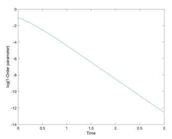
    Exponential aggregation for τ>0, N=4 and d=2

    .

    In the part, we provide four lemmas for the emergent dynamics of (16) following the strategy in [10].

    Lemma 3.2. Let {zj} be a global solution to (16). Then we have

    ddtzizsj22κ0Rezτczτ+sc,zizsjκ0zizsj2(Rezτc,zi+Rezτ+sc,zsj)2κ0N(Rezizsj,zτizτ+sjzizsj2),

    for all i,jN and ts+τ.

    Proof. We set

    zsj(t)=zj(ts),jN.

    Then, it satisfies

    ˙zsj=κ0Nkj(zτ+skRe(zτ+sk,zsj)zsj). (17)

    It follows from (16)1 and (17) that

    ddt(zizsj)=κ0N(ki(zτkRe(zτk,zi)zi)kj(zτ+skRe(zτ+sk,zsj)zsj))=κ0((zτcRe(zτc,zi)zi)(zτ+scRe(zτ+sc,zsj)zsj))κ0N((zτiRe(zτi,zi)zi)(zτ+sjRe(zτ+sj,zsj)zsj)). (18)

    This yields

    ddtzizsj2=2Rezizsj,ddt(zizsj)=2κ0Rezizsj,zτcRe(zτc,zi)zi2κ0Rezizsj,zτ+scRe(zτ+sc,zsj)zsj2κ0NRezizsj,zτiRe(zτi,zi)zi+2κ0NRezizsj,zτ+sjRe(zτ+sj,zsj)zsj=2κ0Rezsj,zτcRe(zτc,zi)zi2κ0Rezi,zτ+scRe(zτ+sc,zsj)zsj2κ0NRezsj,zτiRe(zτi,zi)zi+2κ0NRezi,zτ+sjRe(zτ+sj,zsj)zsj=2κ0(Rezτc,ziRezsj,zi+Rezτ+sc,zsjRezi,zsjRezsj,zτcRezi,zτ+sc)2κ0N(Rezτi,ziRezsj,zi+Rezi,zsjRezτ+sj,zsjRezsj,zτiRezi,zτ+sj). (19)

    On the other hand, we have

    zizsj2=2(1Rezi,zsj),i.e.,Rezi,zsj=112zizsj2. (20)

    We combine (19) and (20) to obtain

    ddtzizsj2=2κ0(Rezτc,zi+Rezτ+sc,zsjRezsj,zτcRezi,zτ+sc)κ0zizsj2(Rezτc,zi+Rezτ+sc,zsj)2κ0N(Rezτi,zi+Rezτ+sj,zsjRezsj,zτiRezi,zτ+sj)+κ0Nzizsj2(Rezτi,zi+Rezτ+sj,zsj)=2κ0Rezτczτ+sc,zizsjκ0zizsj2(Rezτc,zi+Rezτ+sc,zsj)2κ0NRezizsj,zτizτ+sj+κ0Nzizsj2(Rezτi,zi+Rezτ+sj,zsj). (21)

    Finally, relation (21) and |z,w|zw yield desired estimate.

    Lemma 3.3. Let {zj} be a global solution to (16). Then we have following relation for suitable positive numbers s,u,t:

    |zi(t)zsj(t)2Rezui(t)zu+sj(t),zi(t)zsj(t)|2uκ0suptu<v<t(zi(v)zsj(v)+zτc(v)zτ+sc(v))zi(t)zsj(t)+2uκ0Nsuptu<v<t(zi(v)zsj(v)+zτi(v)zτ+sj(v))zi(t)zsj(t).

    Proof. Note that

    |zi(t)zsj(t)2Rezui(t)zu+sj(t),zi(t)zsj(t)|=|Re(zi(t)zsj(t)2zui(t)zu+sj(t),zi(t)zsj(t))|.

    We integrate (18) on the interval [tu,t] and take the inner product of the resulting relation and zi(t)zsj(t) as in [10] to find

    |Re(zi(t)zsj(t)2zui(t)zu+sj(t),zi(t)zsj(t))||zi(t)zsj(t)2zui(t)zu+sj(t),zi(t)zsj(t)|2uκ0suptu<v<t(zi(v)zsj(v)+zτc(v)zτ+sc(v))zi(t)zsj(t)+2uκ0Nsuptu<v<t(zi(v)zsj(v)+zτi(v)zτ+sj(v))zi(t)zsj(t).

    For an emergent dynamics, we introduce a modified ensemble diameter as follows:

    D0,τ(t):=maxi,jzi(t)zτj(t). (22)

    Lemma 3.4. Let {zj} be a global solution to (16). Then, the functional (22) satisfies

    ddtD0,τ(t)κ0zτcz2τcκ0D0,τ(t)2(2D0,τ(t)22D0,τ(tτ)22)+4κ20τ(N+1)N2(supt2τ<v<tD0,τ(v)).

    Proof. In Lemma 3.3, we set s=τ and take s,u=τ. Since inequalities in Lemma 3.3 and Lemma 3.4 are similar to estimates in Lemma 4.1 and 4.2 in [10], we can derive the same result. The only difference is that we have terms involving real parts, but it can be estimated in the same way as [10] since

    1Re(zi,zτc)=Re(1zi,zτc)=1NNk=1Re(1zi,zτk)=1NNk=1zizτk22D0,τ(t)22.

    We set

    Δτzj(t)=zj(t)zτj(t).

    In order to control the term zτcz2τc2 appearing in Lemma 3.4, we give the following estimate for Δτzj.

    Lemma 3.5. Let {zj} be a global solution to (16). Then, the functional Δτzj satisfies

    Δτzj(t)2κ0τ(N1N).

    Proof. Note that

    zj(t)zτj(t)=zj(t)zj(tτ)=ttτ˙zj(s)ds,

    This yields

    ttτ˙zj(s)ds=ttτ(κ0Nkj(zτkRe(zτk,zj)zj))dsttτκ0Nkj(zτkRe(zτk,zj)zj)dsttτκ0Nkj(zτk+|Re(zτk,zj)|zj)dsttτκ0Nkj2ds=2κ0τ(N1N).

    Now we are ready to provide a proof of our first main result.

    In this part, we present our first result on the complete aggregation by combining all the estimates in Lemma 3.2 - Lemma 3.5 in two steps. We will briefly sketch the proof, since in the next section, we will provide more general statement and its proof.

    Step A (Existence of a trapping set): First, we claim

    D0,τ(t)<12,t0.

    Proof. We first estimate D0,τ(t) in an interval [τ,2τ]. Next, we define a set

    T:={t(2τ,):D0,τ(t)<12},

    and proceed the proof using Lipschitz continuity of D0,τ(t) in order to show supT=.

    Note that

    ddtD0,τ(t)κ08κ02D0,τ(t)(2D0,τ(t)22D0,τ(tτ)22)+4κ20τ(N+1)N2supt2τ<v<tD0,τ(v)<κ087κ08D0,τ(t)+κ018<κ047κ08D0,τ(t).

    This yields

    D0,τ(t)max(D0,τ(0),κ047κ08)<12.

    Step B (Key step): We claim

    limtzi(t)zj(t)=0.

    For this, we define a Lyapunov functional E: for Z=(z1,,zN),

    Eij(t):=zi(t)zj(t)2+γttτzi(s)zj(s)2ds,

    where γ is a positive constant. Then, one has

    ddtEij(t)=ddtzi(t)zj(t)2+γzi(t)zj(t)2γzτi(t)zτj(t)27κ04zizj2+2κ0Nzizjzτizτj+2κ0Nzizj2+γzi(t)zj(t)2γzτi(t)zτj(t)2.

    Here, for the computation of ddtzizj2, we used Lemma 3.2 with s=0, and the fact that Rezi+zj,zτc>74 when D0,τ(t)<12(see the proof of Lemma 3.4).

    By applying Young's inequality, we have

    ddtEij(t)7κ04zizj2+κ0Nzizj2+κ0Nzτizτj2+2κ0Nzizj2+γzi(t)zj(t)2γzτi(t)zτj(t)2.

    Now we set γ=κ0N to get

    ddtEij(t)[7κ04+4κ0N]zizj25κ012zizj20,

    since N3. This leads to

    5κ0120zi(s)zj(s)2dsEij(0).

    Using the boundedness of ˙zj for all j, we can apply Barbalat's lemma to obtain the desired result.

    In this subsection, we consider the situation in which the coupling gain pair is close to Stuart-Landau coupling gain pair:

    ˜κ:=κ02+κ1,|˜κ|1.

    Note that

    ˙zj=κ0Nkj(zj,zjzτkzτk,zjzj)+κ1Nkj(zj,zτkzτk,zj)zj=κ0Nkj(zj,zjzτkzτk,zjzj)+κ1Nkj(zj,zτkzτk,zj)zjκ02Nkj(zj,zτkzτk,zj)zj+κ02Nkj(zj,zτkzτk,zj)zj=κ0Nkj(zτkRe(zτk,zj)zj)+˜κNkj(zj,zτkzτk,zj)zj. (23)

    We substitute κ1=˜κκ02 into (23) to get

    {˙zj=κ0Nkj(zj,zjzτkRe(zτk,zj)zj)+˜κNkj(zj,zτkzτk,zj)zj,t>0,zj(t)=φj(t)HSd1,τt0. (24)

    By straightforward calculation, one has

    ddtzizsj2˙zi˙zjs,zizsj+zizsj,˙zi˙zjs=2Re˙zi˙zjs,zizsj=2κ0Rezτczτ+sc,zizsjκ0zizsj2(Rezτc,zi+Rezτ+sc,zsj)2κ0N(Rezizsj,zτizτ+sjzizsj2(Rezτi,zi+Rezτ+sj,zj)2)+4˜κImzi,zsjIm(zτc,zizτ+sc,zsj)+4˜κNImzi,zsjIm(zi,zτizsj,zτ+sj)2κ0Rezτczτ+sc,zizsjκ0zizsj2(Rezτc,zi+Rezτ+sc,zsj)2κ0N(Rezizsj,zτizτ+sjzizsj2)+4|˜κ|zizsj(zτczτ+sc+zizsj)+4N|˜κ|zizsj(zizsj+zτizτ+sj). (25)

    For the second inequality (25), we use the triangle inequality,

    z=w=1|Imz,w|=|Im(z,w1)|=|Imz,wz|zw,

    and similar arguments in the proof of Lemma 3.3 to derive

    |zi(t)zsj(t)2Rezui(t)zu+sj(t),zi(t)zsj(t)|2uκ0suptu<v<t(zi(v)zsj(v)+zτc(v)zτ+sc(v))zi(t)zsj(t)+2uκ0Nsuptu<v<t(zi(v)zsj(v)+zτi(v)zτ+sj(v))zi(t)zsj(t)2u|˜κ|suptu<v<t(2zi(v)zsj(v)+zτc(v)zτ+sc(v))zi(t)zsj(t)+2u|˜κ|Nsuptu<v<t(2zi(v)zsj(v)+zτi(v)zτ+sj(v))zi(t)zsj(t). (26)

    Theorem 3.6. Suppose system parameters and initial data satisfy

    κ0>0,|˜κ|<9256κ0,C1τ<18,N3,φj(t)=1,supτt0D(Z(t))<18,Ωj0,jN,

    where C1:=2(N1N)(κ0+|˜κ|), and let {zj} be a global solution to (24). Then complete aggregation emerges asymptotically:

    limtzi(t)zj(t)=0,i,jN.

    Proof. We leave its detailed proof in Section 3.2.2.

    In this part, we provide several a priori estimates.

    Lemma 3.7. Let {zj} be a global solution to (24). For t2τ, we have following inequality:

    ddtD0,τ(t)κ0zτcz2τcκ02D0,τ(t)(2D0,τ(t)22D0,τ(tτ)22)+2κ0τNsupt2τ<v<tD0,τ(v)(2κ0(N+1N)+3|˜κ|(N+1N))+4|˜κ|N+1Nsupt2τ<v<tD0,τ(v). (27)

    Proof. We set s=τ in the inequality (25) to find

    ddtzizτj22κ0Rezτcz2τc,zizτjκ0zizτj2(Rezτc,zi+Rez2τc,zτj)2κ0N(Rezizτj,zτiz2τjzizτj2)+4|˜κ|zizτj(zτcz2τc+zizτj)+4N|˜κ|zizτj(zizτj+zτiz2τj).

    In the inequality (26), we set

    u=τands=τ

    to get

    |zi(t)zτj(t)2Rezτi(t)z2τj(t),zi(t)zτj(t)|2τκ0suptτ<v<t(zi(v)zτj(v)+zτc(v)z2τc(v))zi(t)zτj(t)+2τκ0Nsuptτ<v<t(zi(v)zτj(v)+zτi(v)z2τj(v))zi(t)zτj(t)+2τ|˜κ|suptτ<v<t(2zi(v)zτj(v)+zτc(v)z2τc(v))zi(t)zτj(t)+2τ|˜κ|Nsuptτ<v<t(2zi(v)zτj(v)+zτi(v)z2τj(v))zi(t)zτj(t).

    For a fixed t, there exist it and jt such that

    D0,τ(t)=zitzτjt.

    Then, for t2τ, one has

    ddtD0,τ(t)2=ddtzitzτjt22κ0zτcz2τcD0,τ(t)κ0D0,τ(t)2(Rezτc,zi+Rez2τc,zτj)+2κ0τND0,τ(t)supt2τ<v<tD0,τ(v)(4κ0+4κ0N+6|˜κ|+6|˜κ|N)+8|˜κ|D0,τ(t)supt2τ<v<tD0,τ(t)+8|˜κ|ND0,τ(t)supt2τ<v<tD0,τ(t).

    Hence, one has

    ddtD0,τ(t)κ0zτcz2τcκ02D0,τ(t)(Rezτc,zi+Rez2τc,zτj)+κ0τNsupt2τ<v<tD0,τ(v)(4κ0+4κ0N+6|˜κ|+6|˜κ|N)+4|˜κ|(N+1)Nsupt2τ<v<tD0,τ(t)κ0zτcz2τcκ02D0,τ(t)(2D0,τ(t)22D0,τ(tτ)22)+κ0τNsupt2τ<v<tD0,τ(v)(4κ0+4κ0N+6|˜κ|+6|˜κ|N)+4|˜κ|supt2τ<v<tD0,τ(v)+4|˜κ|Nsupt2τ<v<tD0,τ(v)=κ0zτcz2τcκ02D0,τ(t)(2D0,τ(t)22D0,τ(tτ)22)+2κ0τNsupt2τ<v<tD0,τ(v)(N+1N)(2κ0+3|˜κ|)+4|˜κ|(N+1N)supt2τ<v<tD0,τ(v).

    Lemma 3.8. Let {zj} be a global solution to (24). Then, one has

    zi(t)zτi(t)C1τ.

    Suppose system parameters and initial data satisfy

    κ0>0,|˜κ|<9256κ0,C1τ<18,N3,φj(t)=1,supτt0D(Z(t))<18,Ωj0,jN,

    and let {zj} be a solution of system (24). Then, the proof consists of two steps.

    Step A (Existence of a trapping set): We claim

    D0,τ(t)<12,t0. (28)

    Proof of (28): We follow the same arguments as in [10]. For this, we divide the estimate into three time intervals:

    0tτ,τt2τandt2τ.

    Step A.1 (Estimate in the time-interval [0,τ]): By triangle inequality, we have

    zi(t)zτj(t)zi(t)zτi(t)+zτi(t)zτj(t)C1τ+D(Z(tτ))<14.

    Step A.2 (Estimate in the time-interval [τ,2τ]): Similar to Step A, we use triangular inequality to get

    zi(t)zτj(t)zi(t)zτi(t)+zτi(t)zτj(t)C1τ+D(Z(tτ)).

    However, since

    zi(t)zj(t)zi(t)zτi(t)+zτi(t)zj(t)C1τ+14<38,

    one has

    D(Z(tτ))<38.

    Therefore, we give

    zi(t)zτj(t)<12.

    Step A.3 (Estimate in the time-interval [2τ,)): By (27), one has

    ddtD0,τ(t)κ0zτcz2τcκ02D0,τ(t)(2D0,τ(t)22D0,τ(tτ)22)+2κ0τNsupt2τ<v<tD0,τ(v)(N+1N)(2κ0+3|˜κ|)+4|˜κ|(N+1N)supt2τ<v<tD0,τ(v)κ08κ02D0,τ(t)(2D0,τ(t)22D0,τ(tτ)22)+3κ04Nsupt2τ<v<tD0,τ(v)+4|˜κ|N+1Nsupt2τ<v<tD0,τ(v).

    Here, we used

    zτcz2τcC1τ<18,(N+1N)(4κ0+6|˜κ|)<6(N+1)N(κ0+|˜κ|)3(N+1)N1C16C1

    for N3.

    Next we claim:

    D0,τ(t)<12,t2τ.

    For a proof, we define a set T as

    T:={t(2τ,):D0,τ(t)<12},

    and proceed the proof using Lipschitz continuity of D0,τ(t) as in [10]. The only difference is the estimate of ddtD0,τ(t). By direct estimates, one has

    ddtD0,τ(t)κ08κ02D0,τ(t)(2D0,τ(t)22D0,τ(tτ)22)+3κ04Nsupt2τ<v<tD0,τ(v)+supt2τ<v<tD0,τ(v)(4|˜κ|+4|˜κ|N)<κ087κ08D0,τ(t)+κ08+83|˜κ|=(κ04+83|˜κ|)7κ08D0,τ(t).

    Hence, it follows from |˜κ|<9256κ0 that

    κ04+83|˜κ|7κ08<12,D0,τ(t)max{D0,τ(0),κ04+83|˜κ|7κ08}<12.

    In this way, we verified claim (28).

    Step B (Zero convergence of modified diameter): We claim

    limtzi(t)zj(t)=0. (29)

    The proof is similar to Theorem 3.1 of [10] with a slight difference. We present main steps that involve such differences. We put s=0 in (25) to get

    ddtzizj2κ0zizj2(Rezτc,zi+Rezτc,zj)2κ0N(Rezizj,zτizτjzizj2)+4|˜κ|zizj2+4N|˜κ|zizj(zizj+zτizτj).

    Next, we define a Lyapunov functional Eij for Z=(z1,,zN) and i,jN:

    Eij(t):=zi(t)zj(t)2+γttτzi(s)zj(s)2ds,

    where γ is a positive constant. Then, one has

    ddtEij(t)=ddtzi(t)zj(t)2+γzi(t)zj(t)2γzτi(t)zτj(t)27κ04zizj2+2κ0Nzizjzτizτj+2κ0Nzizj2+4|˜κ|zizj2+4N|˜κ|zizj(zizj+zτizτj)+γzi(t)zj(t)2γzτi(t)zτj(t)2.

    By Young's inequality, we have

    ddtEij(t)7κ04zizj2+κ0Nzizj2+κ0Nzτizτj2+2κ0Nzizj2+4|˜κ|zizj2+4|˜κ|Nzizj2+2|˜κ|N(zizj2+zτizτj2)+γzi(t)zj(t)2γzτi(t)zτj(t)2=(74κ0+κ0N+2κ0N+4|˜κ|+4|˜κ|N+2|˜κ|N+γ)zizj2+(κ0Nγ+2|˜κ|N)zτizτj2.

    Now, we set

    γ=κ0N+2|˜κ|N.

    Then, we have

    ddtEij(t)(74κ0+κ0N+2κ0N+4|˜κ|+4|˜κ|N+2|˜κ|N+γ)zizj2=(74κ0+4κ0N+4|˜κ|+8|˜κ|N)zizj2.

    For N3 and |˜κ|<116κ0, we have

    74κ0+4κ0N+4|˜κ|+8|˜κ|N<0.

    Here we set

    β=(74κ0+4κ0N+4|˜κ|+8|˜κ|N)

    to obtain

    ddtEij(t)βzizj2.

    This yields

    Eij(t)Eij(0)βt0zi(s)zj(s)2ds

    which is equivalent to

    Eij(t)+βt0zi(s)zj(s)2dsEij(0).

    It follows from definition of Eij that

    Eij0.

    Finally, we have

    βt0zi(s)zj(s)2dsEij(0).

    By letting t, one has

    β0zi(s)zj(s)2dsEij(0).

    It follows from the boundedness of ˙zj for all j that

    sup0t<|ddtzi(t)zj(t)2|<.

    This means zi(s)zj(s) is uniformly continuous. Hence, we can apply Barbalat's lemma to obtain the desired estimate (29).

    In this section, we study the practical aggregation of the LHS model.

    In this subsection, we set

    aij1,Ωj0,i,jN.

    In this case, system (1) becomes

    {˙zj=κ0Nkj(zj,zjzτkzτk,zjzj)+κ1Nkj(zj,zτkzτk,zj)zj,t>0,zj(t)=φj(t)Cd,τt0,jN. (30)

    For handy notation, we set

    Gij:=zi,zj,Gτij:=zτi,zj,Lij:=1Gij,Lτij:=1Gτij. (31)

    Our third main result is concerned with the practical aggregation. Recall that

    L(t)=maxi,j|1zi(t),zj(t)|.

    Theorem 4.1. Suppose coupling gains and initial data satisfy

    2|κ1|<κ0,L(0)<12|κ1|κ0,

    and let {zj} be a global solution to (24). Then, system (24) exhibits the practical synchronization:

    limτ0lim suptL(t)=0.

    Proof. We leave its proof in Section 4.1.2.

    In this part, we provide several lemmas to be crucially used in the proof of Theorem 4.1.

    Lemma 4.2. Let {zj} be a global solution to (31). Then, Gij satisfies

    ddtGij=κ0Nki(Gτkj¯GτkiGij)+κ0Nkj(¯GτkiGτkjGij)+κ1Nki(Gτki¯Gτki)Gij+κ1Nkj(¯GτkjGτkj)Gij.

    Proof. By direct calculation, one has

    ddtGij=˙zi,zj+zi,˙zj=κ0Nki(zi,zizτkzτk,zizi)+κ1Nki(zi,zτkzτk,zi)zi,zj+zi,κ0Nkj(zj,zjzτkzτk,zjzj)+κ1Nkj(zj,zτkzτk,zj)zj=κ0Nki(zτk,zj¯zτk,zizi,zj)+κ1Nki(¯zi,zτk¯zτk,zi)zi,zj+κ0Nkj(zi,zτkzτk,zjzi,zj)+κ1Nkj(zj,zτkzτk,zj)zi,zj=κ0Nki(Gτkj¯GτkiGij)+κ0Nkj(¯GτkiGτkjGij)+κ1Nki(Gτki¯Gτki)Gij+κ1Nkj(¯GτkjGτkj)Gij.

    Lemma 4.3. Let ACd×d and vCd be given matrix and vector, respectively. Then, one has

    AvAFv,

    where is a vector norm in Cd and F is the Frobenius norm defined by AF:=tr(AA).

    Proof. We set the componentwise form of A and v as follows:

    A:=[A]αβandv:=[v]γ,

    where 1α,β,γd. By the Cauchy-Schwarz inequality, we have

    |[Av]α|=|dβ=1[A]αβ[v]β|dβ=1[ˉA]αβ[A]αβdβ=1[ˉv]β[v]β,

    Thus, one has

    Av2=dα=1|[Av]α|2(dα,β=1[ˉA]αβ[A]αβ)(dβ=1[ˉv]β[v]β)=A2Fv2,

    and this yields the desired result.

    Lemma 4.4. Let {zj} be a global solution to (30). Then Lij in (31) satisfies

    |Lij(t)Lτij(t)|τC2,

    where the positive constant C2 is given by

    C2:=2(N1)N(κ0+|κ1|).

    Proof. By the Cauchy-Schwarz inequality, we have

    |Lij(t)Lτij(t)|=|zizτi,zj|zizτizj.

    Note that zj=1. By Lemma 3.8, we have

    zizτiτ(2N1N(κ0+|κ1|)).

    Lemma 4.5. Let {zj} be a global solution to (30). Then, |Lij| satisfies

    ddt|Lij|22κ0NNk=1|Lij|2(Re(zτk,zi+zj)+4|κ1||Lij|(|Lci|+|Lcj|+2C2τ)+|Lij|8C2τN(κ0+|κ1|)+|Lij|24κ0C2τN.

    Proof. We use (30) to get

    ddtGij=κ0Nki(Gτkj¯GτkiGij)+κ0Nkj(¯GτkiGτkjGij)+κ1Nki(GτkiGij¯GτkiGij)+κ1Nkj(¯GτkjGijGτkjGij)=κ0NNk=1(Gτkj¯GτkiGij+¯GτkiGτkjGij)+κ1NNk=1(GτkiGij¯GτkiGij+¯GτkjGijGτkjGij)κ0N(Gτij¯GτiiGij+¯GτjiGτjjGij)κ1N(GτiiGij¯GτiiGij+¯GτjjGijGτjjGij)=κ0NNk=1(2Lτkj¯Lτki)Lij+2iκ1NNk=1(ImLτkjImLτki)(1Lij)κ0N(2LijLτij¯Lτji+Lτjj+¯Lτii¯LτiiLijLτjjLij)2iκ1N(1Lij)(ImLτjjImLτii)

    Thus, we have

    ddt|Lij|2=ddt(LijˉLij)=˙Lij¯Lij+Lij˙¯Lij=ddtzi,zj(1zj,zi)+(1zi,zj)(ddtzj,zi)=Lji(κ0NNk=1(2Lτkj¯Lτki)Lij+2iκ1NNk=1(ImLτkjImLτki)(1Lij)κ0N(2LijLτij¯Lτji+Lτjj+¯Lτii¯LτiiLijLτjjLij)2iκ1N(1Lij)(ImLτjjImLτii))Lij(κ0NNk=1(2Lτki¯Lτkj)Lji+2iκ1NNk=1(ImLτkiImLτkj)(1Lji)κ0N(2LjiLτji¯Lτij+Lτii+¯Lτjj¯LτjjLjiLτiiLji)2iκ1N(1Lji)(ImLτiiImLτjj))=κ0NNk=1LijLji(Lτkj+¯Lτkj+Lτki+¯Lτki4)+2iκ1NNk=1(LijLji)(ImLτkjImLτki)+κ0N(4LijLji+(Lτij¯Lτji+Lτjj+¯Lτii)Lji+(Lτji¯Lτij+Lτii+¯Lτjj)Lij(¯Lτii+Lτjj+¯Lτjj+Lτii)LijLji)+2iκ1N(LijLji)(ImLτiiImLτjj).

    Note that

    LijLji=(1zi,zj)(1zj,zi)=|Lij|2and¯Lij=Lji.

    So we have

    ddt|Lij|2=2κ0NNk=1|Lij|2(ReLτki+ReLτkj2)+4κ1NNk=1ImLij(ImLτkiImLτkj)+κ0N(4|Lij|2+2Re((Lτji¯Lτij+Lτii+¯Lτjj)Lij)2(Re(Lτii+Lτjj)|Lij|2))4κ1NImLijIm(LτiiLτjj).

    Note that the last two terms of the right hand side in above equation goes to zero as τ goes to 0.

    Step A: Note that

    zizj2=|2(1Re(zi,zj)|2|Lij|,

    By Lemma 4.4, we have for any i,

    |Lτii|τC2.

    Since Lii=0, one has

    |4κ1NImLijIm(LτiiLτjj)|=4|κ1|N|Lij|Im(zi,zτizj,zτj)|=4|κ1|N|Lij|Im(zizj,zτi+zj,zτizτj)|4|κ1|N|Lij|(|Lτii|+|Lτjj|)8C2|κ1|τN|Lij|.

    Step B: Next, we analyze the term

    A:=κ0N(4|Lij|2+2Re((Lτji¯Lτij+Lτii+¯Lτjj)Lij)2(Re(Lτii+Lτjj)|Lij|2)=κ0N(4|Lij|2+2Re((LτjiLij¯LτijLij)=:A1+2Re(LτiiLij+¯LτjjLij)2(Re(Lτii+Lτjj)|Lij|2=:A2). (32)

    In the sequel, we estimate Ai,i=1,2 as follows.

    (Estimate of A2): By direct estimate, one has

    A22|LτiiLij|+2|¯LτjjLij|+2((|Lτii|+|Lτjj|)|Lij|2)2|Lij|(|Lτii|+|¯Lτjj|)+2|Lij|2(|Lτii|+|Lτjj|)4C2τ|Lij|+4C2τ|Lij|2. (33)

    On the other hand, note that

    |Lij|2ReLτjiLij=Re|Lij|2ReLτjiLij=Re((LjiLτji)Lij)|((LjiLτji)Lij)|=|LjiLτji||Lij|C2τ|Lij|

    (Estimate of A1): Similarly, by Lemma 4.4, one has

    |Lij|2ReLij¯Lτij=Re(|Lij|2Lij¯Lτij)=Re(LijLjiLij¯Lτij)|Lij||Lji¯Lτij|C2τ|Lij|.

    Thus, we have

    A1=4|Lij|2+2Re((LτjiLij¯LτijLij)=2(|Lij|2+|Lij|2ReLτjiLijRe¯LτijLij)4C2τ|Lij|. (34)

    In (32), we combine all the estimate (33) and (34) to find

    A=κ0N(A1+A2)4κ0C2τN(2|Lij|+|Lij|2),

    and

    κ0N(4|Lij|2+2Re((Lτji¯Lτij+Lτii+¯Lτjj)Lij)2(Re(Lτii+Lτjj)|Lij|2))4κ1NImLijIm(LτiiLτjj)|Lij|8C2|κ1|τ+8C2κ0τN+|Lij|24κ0C2τN.

    Step C: Finally, we analyze the term

    2κ0NNk=1|Lij|2(ReLτki+ReLτkj2)+4κ1NNk=1ImLij(ImLτkiImLτkj).

    By direct calculation, we have

    2κ0NNk=1|Lij|2(ReLτki+ReLτkj2)+4κ1NNk=1ImLij(ImLτkiImLτkj)=2κ0NNk=1|1zi,zj|2(Re(1zτk,zi+1zτk,zj2)+4κ1NNk=1Im(1zi,zj)(Im(1zτk,zi1+zτk,zj)=2κ0NNk=1|1zi,zj|2(Re(zτk,zi+zj)+4κ1NNk=1Im(zi,zj)(Im(zτk,zizj).

    Note that

    4κ1NNk=1Im(zi,zj)(Im(zτk,zizj)=4κ1Im(zi,zj)(Im(zτc,zizj)4|κ1||Lij|(|Lτci|+|Lτcj|)4|κ1||Lij|(|Lci|+|Lcj|+2C2τ),

    and so

    2κ0NNk=1|1zi,zj|2(Re(zτk,zi+zj)+4κ1NNk=1Im(zi,zj)(Im(zτk,zizj)2κ0NNk=1|1zi,zj|2(Re(zτk,zi+zj)+4|κ1||Lij|(|Lci|+|Lcj|+2C2τ).

    Step D: We collect all the estimates in Step A - Step C to find

    ddt|Lij|2=2κ0NNk=1|Lij|2(ReLτki+ReLτkj2)+4κ1NNk=1ImLij(ImLτkiImLτkj)+κ0N(4|Lij|2+2Re((Lτji¯Lτij+Lτii+¯Lτjj)Lij)2(Re(Lτii+Lτjj)|Lij|2)4κ1NImLijIm(LτiiLτjj)2κ0NNk=1|Lij|2(Re(zτk,zi+zj)+4|κ1||Lij|(|Lci|+|Lcj|+2C2τ)+|Lij|8C2|κ1|τ+8C2κ0τN+|Lij|24κ0C2τN.

    We set

    L(t)=maxi,j|Lij|.

    Then, for each time t, there exists it and jt by which the maximum is attained, i.e.

    L(t)=|1zit,zjt|. (35)

    Now we want to obtain the dynamics of L(t).

    Lemma 4.6. Let {zj} be a global solution to (24). Then, the functional L(t) in (35) satisfies

    ddtL(t)2κ0L(t)2+(2κ0+2C2κ0τ+4|κ1|+2C2κ0τN)L(t)+(4C2|κ1|τ+4C2τN(κ0+|κ1|)).

    Proof. It follows from Lemma 4.5 and the fact that |Lci|L(t), we have

    ddtL(t)22κ0L(t)2(Re(zτc,zi+zj)+4|κ1|L(t)(2L(t)+2C2τ)+L(t)8C2|κ1|τ+8C2κ0τN+L(t)24κ0C2τN=(2κ0Re(zτc,zi+zj)+8|κ1|+4C2κ0τN)L(t)2+(8C2|κ1|τ+8C2|κ1|τ+8C2κ0τN)L(t).

    Note that

    Re(zτc,zi+zj)=Re(Lτci+Lτcj)+2.

    Since |Lτci||Lci|+C2τL(t)+C2τ, we have

    ddtL(t)2(2κ0Re(2LτciLτcj)+8|κ1|+4C2κ0τN)L(t)2+(8C2|κ1|τ+8C2|κ1|τ+8C2κ0τN)L(t)
    4κ0L(t)3+(4κ0+4C2κ0τ+8|κ1|+4C2κ0τN)L(t)2+(8C2|κ1|τ+8C2|κ1|τ+8C2κ0τN)L(t).

    Hence we obtain the desired estimate:

    ddtL(t)2κ0L(t)2+(2κ0+2C2κ0τ+4|κ1|+2C2κ0τN)L(t)+(4C2|κ1|τ+4C2τN(κ0+|κ1|)).

    Consider a quadratic polynomial

    f(x)=2κ0x2+(2κ0+2C2κ0τ+4|κ1|+2C2κ0τN)x+(4C2|κ1|τ+4C2τN(κ0+|κ1|))=2κ0(x2(12|κ1|κ0C2τ(N+1N))x+C2τ(2|κ1|κ0(1+1N)+2N)).

    Now we study the practical aggregation as τ0. Here we fix the other variables. Let us assume that 2|κ1|<κ0. Then for a sufficiently small τ, there are two roots of f(x)=0.

    Note that the discriminant Dτ of f(x) is given explicitly as

    Dτ:==C22(N+1N)2τ22C2((1+2|κ1|κ0)N+1N+4N)τ+(12|κ1|κ0)2.

    Note that the constant term (12|κ1|κ0)2 is positive by the assumption so that

    D0>0,

    so Dτ is positive as τ tends to 0. Now, for τ1, we denote two roots by x(τ) and x+(τ) with x(τ)x+(τ). Then we have following property from the phase portrait:

    L(0)<x+(τ)lim suptL(t)x(τ).

    We also obtain

    limτ0x(τ)=0,limτ0x+(τ)=12|κ1|κ0.

    In this subsection, we will study practical aggregation of the system (1). Here we set network topology as {aij} with aij0, for all i,jN.

    {˙zj=Ωjzj+κ0Nkjajk(zj,zjzτkzτk,zjzj)+κ1Nkjajk(zj,zτkzτk,zj)zj,zj(t)=φj(t)Cd,τt0, (36)

    Theorem 4.7. Let {zj} be a global solution to (36) with the following initial condition:

    L(0)<12Nk=1|aikajk|Nk=1(aik+ajk).

    Then, system (36) exhibits the practical aggregation:

    limκ0limτ0lim suptL(t)=0.

    Proof. We leave its proof in Section 4.2.2

    In this part, we provide several a priori estimates to be used in the proof of Theorem 4.7.

    Lemma 4.8. Let {zj} be a global solution to (36). Then Gij in (31) satisfies

    ddtGij=(ΩiΩj)zi,zj+κ0Nkiaik(Gτkj¯GτkiGij)+κ0Nkjajk(¯GτkiGτkjGij)+κ1Nkiaik(Gτki¯Gτki)Gij+κ1Nkjajk(¯GτkjGτkj)Gij.

    Proof. By definition of Gij=zi,zj, one has

    ddtGij=˙zi,zj+zi,˙zj=Ωizi+κ0Nkiaik(zτkzτk,zizi)+κ1Nkiaik(zi,zτkzτk,zi)zi,zj+zi,Ωjzj+κ0Nkjajk(zτkzτk,zjzj)+κ1Nkjajk(zj,zτkzτk,zj)zj=Ωizi,zj+κ0Nkiaik(zτk,zj¯zτk,zizi,zj)+κ1Nkiaik(¯zi,zτk¯zτk,zi)zi,zj+zi,Ωjzj+κ0Nkjajk(zi,zτkzτk,zjzi,zj)+κ1Nkjajk(zj,zτkzτk,zj)zi,zj=(ΩiΩj)zi,zj+κ0Nkiaik(zτk,zj¯zτk,zizi,zj)+κ1Nkiaik(¯zi,zτk¯zτk,zi)zi,zj+κ0Nkjajk(zi,zτkzτk,zjzi,zj)+κ1Nkjajk(zj,zτkzτk,zj)zi,zj=(ΩiΩj)zi,zj+κ0Nkiaik(Gτkj¯GτkiGij)+κ0Nkjajk(¯GτkiGτkjGij)+κ1Nkiaik(Gτki¯Gτki)Gij+κ1Nkjajk(¯GτkjGτkj)Gij.

    which yields the desired estimate.

    Lemma 4.9. Let {zj} be a global solution to (36). Then, one has

    |Lij(t)Lτij(t)|τC3,

    where the positive constant C3 is given by

    C3:=maxiΩi+2A(N1)(κ0+|κ1|)N.

    Proof. By the Cauchy-Schwarz inequality, we have

    |Lij(t)Lτij(t)|=|zizτi,zj|zizτizj=zizτi.

    On the other hand, we have

    zi(t)zτi(t)=ttτ˙zi(s)dsttτΩizi+κ0Nkiaik(zi,zizτkzτk,zizi)+κ1Nkiaik(zi,zτkzτk,zi)zidsτ(Ωi+ki2aik(κ0+|κ1|)N).

    Now, we set

    A:=maxi,jaij.

    Then, we have

    |Lij(t)Lτij(t)|τ(maxiΩi+2A(N1)(κ0+|κ1|)N).

    We set

    D(Ω):=maxi,jΩiΩj.

    Then by direct calculation, we get the following lemma.

    Lemma 4.10. Let {zj} be a global solution to (36). Then |Lij| satisfies

    ddt|Lij|22|Lij|D(Ω)+2κ0NNk=1|aikajk|(|Lki|+|Lkj|+2τC3)|Lij|+4C3|κ1|τN(aii+ajj)|Lij|2κ0NNk=1(aik+ajk)|Lij|2+2κ0NNk=1(aik(|Lki|+τC3)+ajk(|Lkj|+τC3))|Lij|2+2C3κ0τN(aii+ajj)|Lij|+2C3κ0τN(aii+ajj)(|Lij|2+|Lij|)+4|κ1|NNk=1|Lij|(aik(|Lki|+τC3)+ajk(|Lkj|+τC3)). (37)

    Proof. We use (36) to find

    ddtzi,zj=(ΩiΩj)zi,zj+κ0Nkiaik(Gτkj¯GτkiGij)+κ0Nkjajk(¯GτkiGτkjGij)+κ1Nkiaik(Gτki¯Gτki)Gij+κ1Nkjajk(¯GτkjGτkj)Gij=(ΩiΩj)zi,zj+κ0NNk=1(aik(Gτkj¯GτkiGij)+ajk(¯GτkiGτkjGij))+κ1NNk=1(aik(GτkiGij¯GτkiGij)+ajk(¯GτkjGijGτkjGij))κ0N(aii(Gτij¯GτiiGij)+ajj(¯GτjiGτjjGij))
    κ1N(aii(GτiiGij¯GτiiGij)+ajj(¯GτjjGijGτjjGij))=(ΩiΩj)zi,zj+κ0NNk=1[(ajkaik)Lτkj+(aikajk)¯Lτki+(aik+ajkaik¯LτkiajkLτkj)Lij]+2iκ1NNk=1(ajkImLτkjaikImLτki)(1Lij))2iκ1N(ajjImLτjjaiiImLτii)(1Lij)κ0N(ajjLτjjaiiLτij+aii¯Lτiiajj¯Lτji+(aii+ajj)Lijaii¯LτiiLijajjLτjjLij).

    Thus, we have

    ddt|Lij|2=ddt(Lij¯Lij)=2Re(˙Lij¯Lij)=2Re(ddtzi,zj(1zj,zi))=2Re(Lji[(ΩiΩj)zi,zj+κ0NNk=1{(ajkaik)Lτkj+(aikajk)¯Lτki+(aik+ajkaik¯LτkiajkLτkj)Lij}+2iκ1NNk=1(ajkImLτkjaikImLτki)(1Lij))2iκ1N(ajjImLτjjaiiImLτii)(1Lij)κ0N(ajjLτjjaiiLτij+aii¯Lτiiajj¯Lτji+(aii+ajj)Lijaii¯LτiiLijajjLτjjLij)])2|Lij|D(Ω)2Reκ0NNk=1{(aik+ajkaik¯LτkiajkLτkj)|Lij|2+(aikajk)(¯LτkiLτkj)Lji}+Re2κ0N((aii+ajjaii¯LτiiajjLτjj)|Lij|2+(ajjLτjjaiiLτij+aii¯Lτiiajj¯Lτji)Lji)+4κ1NNk=1(Im(aikLτkiajkLτkj)ImLij4κ1NIm(aiiLτiiajjLτjj)ImLij.

    In the sequel, we prove each term in the R.H.S. of the above relation.

    Step A: By direct calculation, one has

    |4κ1NIm(aiiLτiiajjLτjj)ImLij|=4|κ1|N|Lij||Im(aiiLτiiajjLτjj)|4|κ1|N|Lij|(aii|Lτii|+ajj|Lτjj|)4C3|κ1|τN(aii+ajj)|Lij|.

    Step B: We set

    A:=2κ0NRe((aii+ajjaii¯LτiiajjLτjj)|Lij|2+(ajjLτjjaiiLτij+aii¯Lτiiajj¯Lτji)Lji).

    Then, one has

    A2κ0NRe(aii(LijLτij)Lji+ajj(Lij¯Lτji)Lji)+2C3κ0τN(aii+ajj)(|Lij|2+|Lij|)2C3κ0τN(aii+ajj)|Lij|+2C3κ0τN(aii+ajj)(|Lij|2+|Lij|).

    Step C: We set

    B=2Reκ0NNk=1{(aik+ajkaik¯LτkiajkLτkj)|Lij|2+(aikajk)(¯LτkiLτkj)Lji}2κ0NNk=1(aik+ajk)|Lij|2+2κ0NNk=1(aik(|Lki|+τC3)+ajk(|Lkj|+τC3))|Lij|2+2κ0NNk=1|aikajk|(|Lki|+|Lkj|+2τC3)|Lij|.

    Step D: Note that

    4κ1NNk=1(Im(aikLτkiajkLτkj)ImLij4|κ1|NNk=1|Lij|(aik(|Lki|+τC3)+ajk(|Lkj|+τC3)).

    Step E: We collect all the estimates in Step A - Step D to get

    ddt|Lij|22|Lij|D(Ω)+2κ0NNk=1|aikajk|(|Lki|+|Lkj|+2τC3)|Lij|+4C3|κ1|τN(aii+ajj)|Lij|2κ0NNk=1(aik+ajk)|Lij|2+2κ0NNk=1(aik(|Lki|+τC3)+ajk(|Lkj|+τC3))|Lij|2+2C3κ0τN(aii+ajj)|Lij|+2C3κ0τN(aii+ajj)(|Lij|2+|Lij|)+4|κ1|NNk=1|Lij|(aik(|Lki|+τC3)+ajk(|Lkj|+τC3)).

    Recall that

    L(t):=maxi,jLij.

    Then, for each time t, there exists it and jt by which the maximum is attained:

    L(t)=|1zit,zjt|.

    Then by Lemma 4.10, one has

    ddtL(t)22L(t)D(Ω)+4κ0NNk=1|aikajk|(L(t)+τC3)L(t)+4C3|κ1|τN(aii+ajj)L(t)2κ0NNk=1(aik+ajk)L(t)2+2κ0NNk=1(aik(L(t)+τC3)+ajk(L(t)+τC3))L(t)2+2C3κ0τN(aii+ajj)L(t)+2C3κ0τN(aii+ajj)(L(t)2+L(t))+4|κ1|NNk=1L(t)(aik(L(t)+τC3)+ajk(L(t)+τC3))2κ0NNk=1(aik+ajk)L(t)3
    +(2κ0NNk=1(aik+ajk)+4κ0NNk=1|aikajk|+4C3κ0τNNk=1(aik+ajk)+2C3κ0τN(aii+ajj)+4|κ1|NNk=1(aik+ajk))L(t)2+(2D(Ω)+4C3κ0τNNk=1|aikajk|+(aii+ajj)4C3τN(κ0+|κ1|)+4C3|κ1|τNNk=1(aik+ajk))L(t).

    Then, we have

    ddtL(t)κ0NNk=1(aik+ajk)L(t)2+(κ0NNk=1(aik+ajk)+2κ0NNk=1|aikajk|+2C3κ0τNNk=1(aik+ajk)+C3κ0τN(aii+ajj)+2|κ1|NNk=1(aik+ajk))L(t)+(D(Ω)+2C3κ0τNNk=1|aikajk|+2C3τN(aii+ajj)(κ0+|κ1|)+2C3|κ1|τNNk=1(aik+ajk)).

    Now, we set

    A1:=1NNk=1(aik+ajk),A2:=2NNk=1|aikajk|+2C3τNNk=1(aik+ajk)+C3τN(aii+ajj)+2|κ1|Nκ0Nk=1(aik+ajk),A3:=D(Ω)κ0+2C3τNNk=1|aikajk|+2C3τN(aii+ajj)(1+|κ1|κ0)+2C3|κ1|τNκ0Nk=1(aik+ajk).

    This yields

    ddtLκ0(A1L2(A1A2)L+A3).

    If we impose following conditions:

    τ0andafterthatκ0, (38)

    we obtain

    limκ0limτ0A2=2NNk=1|aikajk|,limκ0limτ0A3=0.

    Since the roots of

    A1x2(A1A2)x+A3=0

    can be expressed as

    x±=A1A2±(A1A2)24A1A32A1.

    If we combine this expression, under the condition (38) we have

    limκ0limτ0x+=12Nk=1|aikajk|Nk=1(aik+ajk),limκ0limτ0x=0.

    By similar arguments with previous result, we have desired estimate.

    In this paper, we have proposed several sufficient frameworks leading to complete aggregation and practical aggregation in terms of initial data, coupling gains and size of time-delay for the LHS model with time-delayed interactions. The LHS model is a complex counterpart of the LS model, and it describes the continuous-time dynamics of the Lohe Hermitian sphere particles on the unit Hermitian sphere. For the SL coupling gain pair with κ1=κ02, the LHS model on Cd can be rewritten as the LS model on R2d. When the coupling gain pair is close to that of the SL coupling gain pair and the corresponding linear flows are the same, we show that the LHS flow with a time-delay tends to complete aggregation asymptotically for some admissible class of initial data and system parameters. For a general network, we also provided a sufficient framework for practical aggregation to the LHS model with respect to time-delay. Even for the LS model on the unit sphere in Euclidean space, the complete aggregation is not known in previous literature, except some weak aggregation estimates such as practical aggregation. We leave this interesting issue for a future work.

    We begin with the generalized Stuart-Landau model on Cd+1:

    dzjdt=((1zj2)Id+1+Ω)zj+κNNk=1(zkzj), (39)

    where zjCd+1 for all jN, Ω is a skew-Hermitian matrix with the size (d+1)×(d+1) and is the identity matrix with the size . Now, we substitute the ansatz:

    into (39) to see

    (40)

    Then, implies

    (41)

    where we used the fact that .

    If we take the real part of (41), one has

    (42)

    where we used the relations:

    Now, we combine (40) and (42) to get

    (43)

    Similarly, we impose on (43) to obtain

    If we put and into the LHS model, then we get the above system. Therefore, the SL coupling gain pair can be obtained by the generalized Stuart-Landau model.


    [1] The Kuramoto model: A simple paradigm for synchronization phenomena. Rev. Mod. Phys. (2005) 77: 137-185.
    [2] Vehicular traffic, crowds and swarms: From kinetic theory and multiscale methods to applications and research perspectives. Math. Models Methods Appl. Sci. (2019) 29: 1901-2005.
    [3] Systemes dequations differentielles d oscillations non lineaires. Rev. Math. Pures Appl. (1959) 4: 267-270.
    [4] A quest toward a mathematical theory of the dynamics of swarms. Math. Models Methods Appl. Sci. (2017) 27: 745-770.
    [5] On the complete phase synchronization for the Kuramoto model in the mean-field limit. Commun. Math. Sci. (2015) 13: 1775-1786.
    [6] A matrix-valued Kuramoto model. J. Stat. Phys. (2020) 178: 595-624.
    [7] Biology of synchronous flashing of fireflies. Nature (1966) 211: 562-564.
    [8]

    J. Byeon, S. -Y. Ha and H. Park, Asymptotic interplay of states and adapted coupling gains in the Lohe Hermitian sphere model, Submitted.

    [9] Time-delayed interactions and synchronization of identical Lohe oscillators. Quart. Appl. Math. (2016) 74: 297-319.
    [10]

    S. -H. Choi and S. -Y. Ha, Large-time dynamics of the asymptotic Lohe model with a small time-delay, J. Phys. A, 48 (2015), 425101 34 pp.

    [11] Complete entrainment of Lohe oscillators under attractive and repulsive couplings. SIAM. J. Appl. Dyn. Syst. (2014) 13: 1417-1441.
    [12] On exponential synchronization of Kuramoto oscillators. IEEE Trans. Automatic Control (2009) 54: 353-357.
    [13] Quaternions in collective dynamics. Multiscale Model. Simul. (2018) 16: 28-77.
    [14] Synchronization and stability for quantum Kuramoto. J. Stat. Phys. (2019) 174: 160-187.
    [15] Synchronization analysis of Kuramoto oscillators. Commun. Math. Sci. (2013) 11: 465-480.
    [16] Synchronization in complex networks of phase oscillators: A survey. Automatica J. IFAC (2014) 50: 1539-1564.
    [17] On the critical coupling for Kuramoto oscillators. SIAM. J. Appl. Dyn. Syst. (2011) 10: 1070-1099.
    [18]

    S. -Y. Ha, D. Kim, D. Kim, H. Park and W. Shim, Emergent dynamics of the Lohe matrix ensemble on a network under time-delayed interactions, J. Math. Phys., 61 (2020), 012702.

    [19] Collective synchronization of classical and quantum oscillators. EMS Surv. Math. Sci. (2016) 3: 209-267.
    [20] On the relaxation dynamics of Lohe oscillators on some Riemannian manifolds. J. Stat. Phys. (2018) 172: 1427-1478.
    [21] Emergent dynamics of Kuramoto oscillators with adaptive couplings: Conservation law and fast learning. SIAM J. Appl. Dyn. Syst. (2018) 17: 1560-1588.
    [22] Synchronization of Kuramoto oscillators with adaptive couplings. SIAM J. Appl. Dyn. Syst. (2016) 15: 162-194.
    [23] Emergent behaviors of Lohe tensor flocks. J. Stat. Phys. (2020) 178: 1268-1292.
    [24] From the Lohe tensor model to the Lohe Hermitian sphere model and emergent dynamics. SIAM J. Appl. Dyn. Syst. (2020) 19: 1312-1342.
    [25]

    J. Hale, Theory of Functional Differential Equations, 2nd ed., Springer-Verlag, New York-Heidelberg, 1977.

    [26]

    V. Jaćimović and A. Crnkić, Low-dimensional dynamics in non-Abelian Kuramoto model on the 3-sphere, Chaos, 28 (2018), 083105.

    [27] State-dependent dynamics of the Lohe matrix ensemble on the unitary group under the gradient flow. SIAM J. Appl. Dyn. Syst. (2020) 19: 1080-1123.
    [28] (1993) Delay Differential Equations with Applications in Population Dynamics. Inc. Boston, MA: Academic Press.
    [29]

    Y. Kuramoto, Self-Entrainment of a Population of Coupled Non-Linear Oscillators, International Symposium on Mathematical Problems in Mathematical Physics, Lecture Notes in Phys., Vol. 39, Springer, Berlin, 1975, 420-422.

    [30]

    M. A. Lohe, Systems of matrix Riccati equations, linear fractional transformations, partial integrability and synchronization, J. Math. Phys., 60 (2019), 072701.

    [31]

    M. A. Lohe, Quantum synchronization over quantum networks, J. Phys. A, 43 (2010), 465301.

    [32]

    M. A. Lohe, Non-abelian Kuramoto models and synchronization, J. Phys. A, 42 (2009), 395101.

    [33] Almost global consensus on the n-sphere. IEEE Trans. Automat. Control (2018) 63: 1664-1675.
    [34]

    C. S. Peskin, Mathematical Aspects of Heart Physiology, Courant Institute of Mathematical Sciences, New York University, New York, 1975.

    [35] (2001) Synchronization: A Universal Concept in Nonlinear Sciences. Cambridge: Cambridge University Press.
    [36] From Kuramoto to Crawford: Exploring the Onset of Synchronization in Populations of Coupled Oscillators. Phys. D (2000) 143: 1-20.
    [37] A lifting method for analyzing distributed synchronization on the unit sphere. Automatica J. IFAC (2018) 96: 253-258.
    [38] A nonlocal continuum model for biological aggregation. Bull. Math. Biol. (2006) 68: 1601-1623.
    [39] Swarming patterns in a two-dimensional kinematic model for biological groups. SIAM J. Appl. Math. (2004) 65: 152-174.
    [40] Collective motion. Phys. Rep. (2012) 517: 71-140.
    [41] Biological rhythms and the behavior of populations of coupled oscillators. J. Theor. Biol. (1967) 16: 15-42.
    [42]

    A. T. Winfree, The Geometry of Biological Time, Springer-Verlag, Berlin-New York, 1980.

    [43] Synchronization of Kuramoto model in a high-dimensional linear space. Phys. Lett. A (2013) 377: 2939-2943.
  • Reader Comments
  • © 2021 the Author(s), licensee AIMS Press. This is an open access article distributed under the terms of the Creative Commons Attribution License (http://creativecommons.org/licenses/by/4.0)
通讯作者: 陈斌, bchen63@163.com
  • 1. 

    沈阳化工大学材料科学与工程学院 沈阳 110142

  1. 本站搜索
  2. 百度学术搜索
  3. 万方数据库搜索
  4. CNKI搜索

Metrics

Article views(1630) PDF downloads(226) Cited by(0)

Figures and Tables

Figures(1)

Other Articles By Authors

/

DownLoad:  Full-Size Img  PowerPoint
Return
Return

Catalog