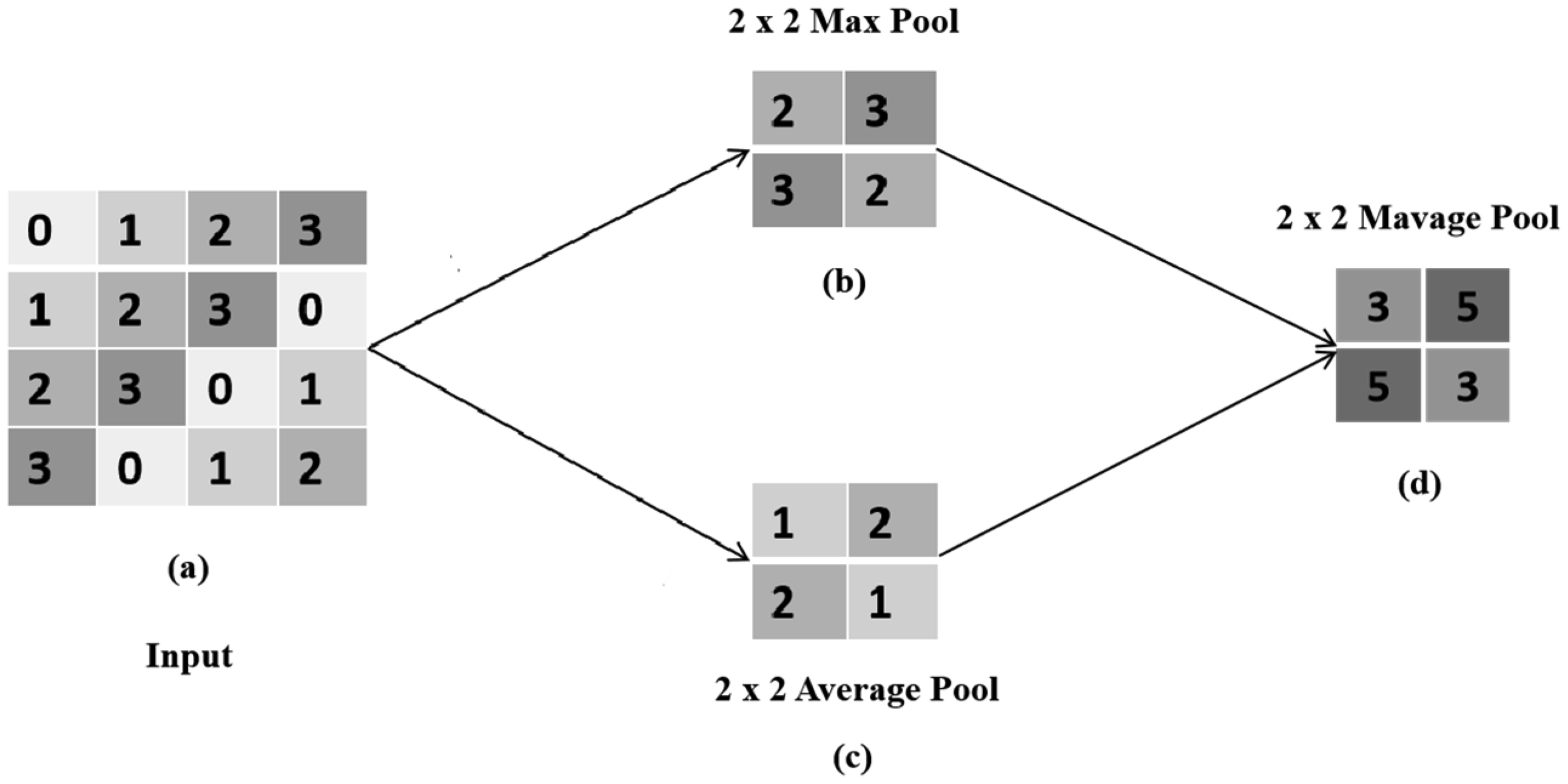
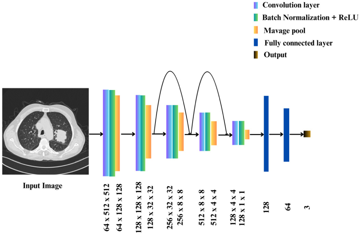
Lung cancer is a deadly disease. An early diagnosis can significantly improve the patient survival and quality of life. One potential solution is using deep learning (DL) algorithms to automate the diagnosis using patient computed tomography (CT) scans. However, the limited availability of training data and the computational complexity of existing algorithms, as well as their reliance on high-performance systems, limit the potential of DL algorithms. To improve early lung cancer diagnoses, this study proposes a low-cost convolutional neural network (CNN) that uses a Mavage pooling technique to diagnose lung cancers.
The DL-based model uses five convolution layers with two residual connections and Mavage pooling layers. We trained the CNN using two publicly available datasets comprised of the IQ_OTH/NCCD dataset and the chest CT scan dataset. Additionally, we integrated the Mavage pooling in the AlexNet, ResNet-50, and GoogLeNet architectures to analyze the datasets. We evaluated the performance of the models based on accuracy and the area under the receiver operating characteristic curve (AUROC).
The CNN model achieved a 99.70% accuracy and a 99.66% AUROC when the scans were classified as either cancerous or non-cancerous. It achieved a 90.24% accuracy and a 94.63% AUROC when the scans were classified as containing either normal, benign, or malignant nodules. It achieved a 95.56% accuracy and a 99.37% AUROC when lung cancers were classified. Additionally, the results indicated that the diagnostic abilities of AlexNet, ResNet-50, and GoogLeNet were improved with the introduction of the Mavage pooling technique.
This study shows that a low-cost CNN can effectively diagnose lung cancers from patient CT scans. Utilizing Mavage pooling technique significantly improves the CNN diagnostic capabilities.
The code is available at: https://github.com/Saintcodded/Mavage-Pooling.git
Citation: Ayomide Abe, Mpumelelo Nyathi, Akintunde Okunade. Lung cancer diagnosis from computed tomography scans using convolutional neural network architecture with Mavage pooling technique[J]. AIMS Medical Science, 2025, 12(1): 13-27. doi: 10.3934/medsci.2025002
Lung cancer is a deadly disease. An early diagnosis can significantly improve the patient survival and quality of life. One potential solution is using deep learning (DL) algorithms to automate the diagnosis using patient computed tomography (CT) scans. However, the limited availability of training data and the computational complexity of existing algorithms, as well as their reliance on high-performance systems, limit the potential of DL algorithms. To improve early lung cancer diagnoses, this study proposes a low-cost convolutional neural network (CNN) that uses a Mavage pooling technique to diagnose lung cancers.
The DL-based model uses five convolution layers with two residual connections and Mavage pooling layers. We trained the CNN using two publicly available datasets comprised of the IQ_OTH/NCCD dataset and the chest CT scan dataset. Additionally, we integrated the Mavage pooling in the AlexNet, ResNet-50, and GoogLeNet architectures to analyze the datasets. We evaluated the performance of the models based on accuracy and the area under the receiver operating characteristic curve (AUROC).
The CNN model achieved a 99.70% accuracy and a 99.66% AUROC when the scans were classified as either cancerous or non-cancerous. It achieved a 90.24% accuracy and a 94.63% AUROC when the scans were classified as containing either normal, benign, or malignant nodules. It achieved a 95.56% accuracy and a 99.37% AUROC when lung cancers were classified. Additionally, the results indicated that the diagnostic abilities of AlexNet, ResNet-50, and GoogLeNet were improved with the introduction of the Mavage pooling technique.
This study shows that a low-cost CNN can effectively diagnose lung cancers from patient CT scans. Utilizing Mavage pooling technique significantly improves the CNN diagnostic capabilities.
The code is available at: https://github.com/Saintcodded/Mavage-Pooling.git

| [1] |
Cruz CSD, Tanoue LT, Matthay RA (2011) Lung cancer: epidemiology, etiology, and prevention. Clin Chest Med 32: 605-644. https://doi.org/10.1016/j.ccm.2011.09.001 
|
| [2] |
Bray F, Ferlay J, Soerjomataram I, et al. (2018) Global cancer statistics 2018: GLOBOCAN estimates of incidence and mortality worldwide for 36 cancers in 185 countries. CA Cancer J Clin 68: 394-424. https://doi.org/10.3322/caac.21492
|
| [3] |
Schabath MB, Cote ML (2019) Cancer progress and priorities: lung cancer. Cancer Epidemiol Biomarkers Prev 28: 1563-1579. https://doi.org/10.1158/1055-9965.EPI-19-0221
|
| [4] |
Yoon SM, Shaikh T, Hallman M (2017) Therapeutic management options for stage III non-small cell lung cancer. World J Clin Oncol 8: 1-20. https://doi.org/10.5306/wjco.v8.i1.1
|
| [5] |
Hoffman RM, Atallah RP, Struble RD, et al. (2020) Lung cancer screening with low-dose CT: a meta-analysis. J Gen Intern Med 35: 3015-3025. https://doi.org/10.1007/s11606-020-05951-7
|
| [6] |
Silvestri GA, Goldman L, Tanner NT, et al. (2023) Outcomes from more than 1 million people screened for lung cancer with low-dose CT imaging. Chest 164: 241-251. https://doi.org/10.1016/j.chest.2023.02.003
|
| [7] |
Shin HJ, Kim MS, Kho BG, et al. (2020) Delayed diagnosis of lung cancer due to misdiagnosis as worsening of sarcoidosis: a case report. BMC Pulm Med 20: 1-4. https://doi.org/10.1186/s12890-020-1105-2
|
| [8] |
Del Ciello A, Franchi P, Contegiacomo A, et al. (2017) Missed lung cancer: when, where, and why?. Diagn Interv Radiol 23: 118-126. https://doi.org/10.5152/dir.2016.16187
|
| [9] |
Friedland B (2009) Medicolegal issues related to cone beam CT. Semin Orthod 15: 77-84. https://doi.org/10.1053/j.sodo.2008.09.010
|
| [10] |
Krupinski EA, Berbaum KS, Caldwell RT, et al. (2010) Long radiology workdays reduce detection and accommodation accuracy. J Am Coll Radiol 7: 698-704. https://doi.org/10.1016/j.jacr.2010.03.004
|
| [11] |
Abujudeh HH, Boland GW, Kaewlai R, et al. (2010) Abdominal and pelvic computed tomography (CT) interpretation: discrepancy rates among experienced radiologists. Eur Radiol 20: 1952-1957. https://doi.org/10.1007/s00330-010-1763-1
|
| [12] |
Jacobsen MM, Silverstein SC, Quinn M, et al. (2017) Timeliness of access to lung cancer diagnosis and treatment: a scoping literature review. Lung cancer 112: 156-164. https://doi.org/10.1016/j.lungcan.2017.08.011
|
| [13] | Sathyakumar K, Munoz M, Singh J, et al. (2020) Automated lung cancer detection using artificial intelligence (AI) deep convolutional neural networks: a narrative literature review. Cureus 12: e10017. https://doi.org/10.7759/cureus.10017 |
| [14] |
Huang S, Yang J, Shen N, et al. (2023) Artificial intelligence in lung cancer diagnosis and prognosis: current application and future perspective. Semin Cancer Biol 89: 30-37. https://doi.org/10.1016/j.semcancer.2023.01.006
|
| [15] |
Ardila D, Kiraly AP, Bharadwaj S, et al. (2019) End-to-end lung cancer screening with three-dimensional deep learning on low-dose chest computed tomography. Nat Med 25: 954-961. https://doi.org/10.1038/s41591-019-0447-x
|
| [16] |
Alrahhal MS, Alqhtani E (2021) Deep learning-based system for detection of lung cancer using fusion of features. Int J Comput Sci Mobile Comput 10: 57-67. https://doi.org/10.47760/ijcsmc.2021.v10i02.009
|
| [17] |
Huang X, Shan J, Vaidya V (2017) Lung nodule detection in CT using 3D convolutional neural networks. 2017 IEEE 14th International Symposium on Biomedical Imaging (ISBI 2017) : 379-383. https://doi.org/10.1109/ISBI.2017.7950542
|
| [18] |
Guo Y, Song Q, Jiang M, et al. (2021) Histological subtypes classification of lung cancers on CT images using 3D deep learning and radiomics. Acad Radiol 28: e258-e266. https://doi.org/10.1016/j.acra.2020.06.010
|
| [19] |
Cui X, Zheng S, Heuvelmans MA, et al. (2022) Performance of a deep learning-based lung nodule detection system as an alternative reader in a Chinese lung cancer screening program. Eur J Radiol 146: 110068. https://doi.org/10.1016/j.ejrad.2021.110068
|
| [20] |
Dunn B, Pierobon M, Wei Q (2023) Automated classification of lung cancer subtypes using deep learning and CT-scan based radiomic analysis. Bioengineering 10: 690. https://doi.org/10.3390/bioengineering10060690
|
| [21] |
de Margerie-Mellon C, Chassagnon G (2023) Artificial intelligence: a critical review of applications for lung nodule and lung cancer. Diagn Interv Imaging 104: 11-17. https://doi.org/10.1016/j.diii.2022.11.007
|
| [22] |
Ahmed SF, Alam MSB, Hassan M, et al. (2023) Deep learning modelling techniques: current progress, applications, advantages, and challenges. Artif Intell Rev 56: 13521-13617. https://doi.org/10.1007/s10462-023-10466-8
|
| [23] |
Zhang J, Xia Y, Zeng H, et al. (2018) NODULe: combining constrained multi-scale LoG filters with densely dilated 3D deep convolutional neural network for pulmonary nodule detection. Neurocomputing 317: 159-167. https://doi.org/10.1016/j.neucom.2018.08.022
|
| [24] | AL-Huseiny MS, Sajit AS (2021) Transfer learning with GoogLeNet for detection of lung cancer. Indones J Electr Eng Comput Sci 22: 1078-1086. https://doi.org/10.11591/ijeecs.v22.i2.pp1078-1086 |
| [25] |
Sakshiwala, Singh MP (2023) A new framework for multi-scale CNN-based malignancy classification of pulmonary lung nodules. J Ambient Intell Human Comput 14: 4675-4683. https://doi.org/10.1007/s12652-022-04368-w
|
| [26] |
Mamun M, Mahmud MI, Meherin M, et al. (2023) LCDctCNN: lung cancer diagnosis of CT scan images using CNN based model. 2023 10th International Conference on Signal Processing and Integrated Networks (SPIN) : 205-212. https://doi.org/10.1109/SPIN57001.2023.10116075
|
| [27] | Krizhevsky A, Sutskever I, Hinton GE (2012) Imagenet classification with deep convolutional neural networks. Adv Neural Inf Process Syst 25. |
| [28] | Hua KL, Hsu CH, Hidayati SC, et al. (2015) Computer-aided classification of lung nodules on computed tomography images via deep learning technique. Onco Targets Ther 8: 2015-2022. https://doi.org/10.2147/OTT.S80733 |
| [29] | Ronneberger O, Fischer P, Brox T (2015) U-net: Convolutional networks for biomedical image segmentation. Medical Image Computing and Computer-Assisted Intervention–MICCAI 2015 . Springer International Publishing 234-241. https://doi.org/10.1007/978-3-319-24574-4_28 |
| [30] |
Gulshan V, Peng L, Coram M, et al. (2016) Development and validation of a deep learning algorithm for detection of diabetic retinopathy in retinal fundus photographs. JAMA 316: 2402-2410. https://doi.org/10.1001/jama.2016.17216
|
| [31] |
Kaul V, Enslin S, Gross SA (2020) History of artificial intelligence in medicine. Gastrointest Endosc 92: 807-812. https://doi.org/10.1016/j.gie.2020.06.040
|
| [32] |
Esteva A, Kuprel B, Novoa RA, et al. (2017) Dermatologist-level classification of skin cancer with deep neural networks. Nature 542: 115-118. https://doi.org/10.1038/nature21056
|
| [33] |
Saouli R, Akil M, Kachouri R (2018) Fully automatic brain tumor segmentation using end-to-end incremental deep neural networks in MRI images. Comput Methods Programs Biomed 166: 39-49. https://doi.org/10.1016/j.cmpb.2018.09.007
|
| [34] |
Lorenzo PR, Nalepa J, Bobek-Billewicz B, et al. (2019) Segmenting brain tumors from FLAIR MRI using fully convolutional neural networks. Comput Methods Programs Biomed 176: 135-148. https://doi.org/10.1016/j.cmpb.2019.05.006
|
| [35] |
Moitra D, Mandal RK (2019) Automated AJCC staging of non-small cell lung cancer (NSCLC) using deep convolutional neural network (CNN) and recurrent neural network (RNN). Health Inf Sci Syst 7: 1-12. https://doi.org/10.1007/s13755-019-0077-1
|
| [36] |
Chaunzwa TL, Hosny A, Xu Y, et al. (2021) Deep learning classification of lung cancer histology using CT images. Sci Rep 11: 1-12. https://doi.org/10.1038/s41598-021-84630-x
|
| [37] |
Anari S, Tataei Sarshar N, Mahjoori N, et al. (2022) Review of deep learning approaches for thyroid cancer diagnosis. Math Probl Eng 2022: 5052435. https://doi.org/10.1155/2022/5052435
|
| [38] |
Painuli D, Bhardwaj S, Köse U (2022) Recent advancement in cancer diagnosis using machine learning and deep learning techniques: a comprehensive review. Comput Biol Med 146: 105580. https://doi.org/10.1016/j.compbiomed.2022.105580
|
| [39] |
Hosseini SH, Monsefi R, Shadroo S (2024) Deep learning applications for lung cancer diagnosis: a systematic review. Multimed Tools Appl 83: 14305-14335. https://doi.org/10.1007/s11042-023-16046-w
|
| [40] |
Aamir M, Rahman Z, Abro WA, et al. (2023) Brain tumor classification utilizing deep features derived from high-quality regions in MRI images. Biomed Signal Proces 85: 104988. https://doi.org/10.1016/j.bspc.2023.104988
|
| [41] |
Sun M, Song Z, Jiang X, et al. (2017) Learning pooling for convolutional neural network. Neurocomputing 224: 96-104. https://doi.org/10.1016/j.neucom.2016.10.049
|
| [42] |
Kumar RL, Kakarla J, Isunuri BV, et al. (2021) Multi-class brain tumor classification using residual network and global average pooling. Multimed Tools Appl 80: 13429-13438. https://doi.org/10.1007/s11042-020-10335-4
|
| [43] |
Zafar A, Aamir M, Mohd Nawi N, et al. (2022) A comparison of pooling methods for convolutional neural networks. Appl Sci 12: 8643. https://doi.org/10.3390/app12178643
|
| [44] |
Nirthika R, Manivannan S, Ramanan A, et al. (2022) Pooling in convolutional neural networks for medical image analysis: a survey and an empirical study. Neural Comput Appl 34: 5321-5347. https://doi.org/10.1007/s00521-022-06953-8
|
| [45] |
Xiong W, Zhang L, Du B, et al. (2017) Combining local and global: rich and robust feature pooling for visual recognition. Pattern Recogn 62: 225-235. https://doi.org/10.1016/j.patcog.2016.08.006
|
| [46] |
Dogan Y (2023) A new global pooling method for deep neural networks: Global average of top-k max-pooling. Trait Signal 40: 577-587. https://doi.org/10.18280/ts.400216
|
| [47] |
Nirthika R, Manivannan S, Ramanan A, et al. (2022) Pooling in convolutional neural networks for medical image analysis: a survey and an empirical study. Neural Comput Applic 34: 5321-5347. https://doi.org/10.1007/s00521-022-06953-8
|
| [48] |
Abuqaddom I, Mahafzah BA, Faris H (2021) Oriented stochastic loss descent algorithm to train very deep multi-layer neural networks without vanishing gradients. Knowledge-Based Systems 230: 107391. https://doi.org/10.1016/j.knosys.2021.107391
|
| [49] |
LeCun Y, Bottou L, Bengio Y, et al. (1998) Gradient-based learning applied to document recognition. Proc IEEE 86: 2278-2324. https://doi.org/10.1109/5.726791
|
| [50] | Sabri N, Hamed HNA, Ibrahim Z, et al. (2020) A comparison between average and max-pooling in convolutional neural network for scoliosis classification. Int J 9. https://doi.org/10.30534/ijatcse/2020/9791.42020 |
| [51] |
Hyun J, Seong H, Kim E (2021) Universal pooling–a new pooling method for convolutional neural networks. Expert Syst Appl 180: 115084. https://doi.org/10.1016/j.eswa.2021.115084
|
| [52] |
Özdemir C (2023) Avg-topk: a new pooling method for convolutional neural networks. Expert Syst Appl 223: 119892. https://doi.org/10.1016/j.eswa.2023.119892
|
| [53] |
Zhou Q, Qu Z, Cao C (2021) Mixed pooling and richer attention feature fusion for crack detection. Pattern Recogn Lett 145: 96-102. https://doi.org/10.1016/j.patrec.2021.02.005
|
| [54] | Hou Q, Zhang L, Cheng MM, et al. (2020) Strip pooling: Rethinking spatial pooling for scene parsing. Proceedings of the IEEE/CVF conference on computer vision and pattern recognition : 4003-4012. |
| [55] | Kareem HF, AL-Husieny MS, Mohsen FY, et al. (2021) Evaluation of SVM performance in the detection of lung cancer in marked CT scan dataset. Indones J Electr Eng Comput Sci 21: 1731-1738. https://doi.org/10.11591/ijeecs.v21.i3.pp1731-1738 |
| [56] | Alyasriy H (2020) The IQ-OTHNCCD lung cancer dataset. Mendeley Data . Available from: https://data.mendeley.com/datasets/bhmdr45bh2/1. Retrieved June 15, 2024 |
| [57] | Hany M Chest CT-scan images dataset (2020). Available from: https://www.kaggle.com/datasets/mohamedhanyyy/chest-ctscan-images. Retrieved June 15, 2024 |
| [58] | He K, Zhang X, Ren S, et al. (2016) Deep residual learning for image recognition. Proceedings of the IEEE conference on computer vision and pattern recognition : 770-778. |
| [59] | Szegedy C, Liu W, Jia Y, et al. (2015) Going deeper with convolutions. Proceedings of the IEEE conference on computer vision and pattern recognition : 1-9. |
| [60] | Paszke A, Gross S, Massa F, et al. (2019) Pytorch: an imperative style, high-performance deep learning library. Adv Neural Inf Process Syst 32. |
Figures(2) / Tables(4)

Ayomide Abe, Mpumelelo Nyathi, Akintunde Okunade. Lung cancer diagnosis from computed tomography scans using convolutional neural network architecture with Mavage pooling technique[J]. AIMS Medical Science, 2025, 12(1): 13-27. doi: 10.3934/medsci.2025002


 DownLoad: