Digital voice assistants (DVAs) are increasingly used to search for health information. However, the quality of information provided by DVAs is not consistent across health conditions. From our knowledge, there have been no studies that evaluated the quality of DVAs in response to diabetes-related queries. The objective of this study was to evaluate the quality of DVAs in relation to queries on diabetes management.
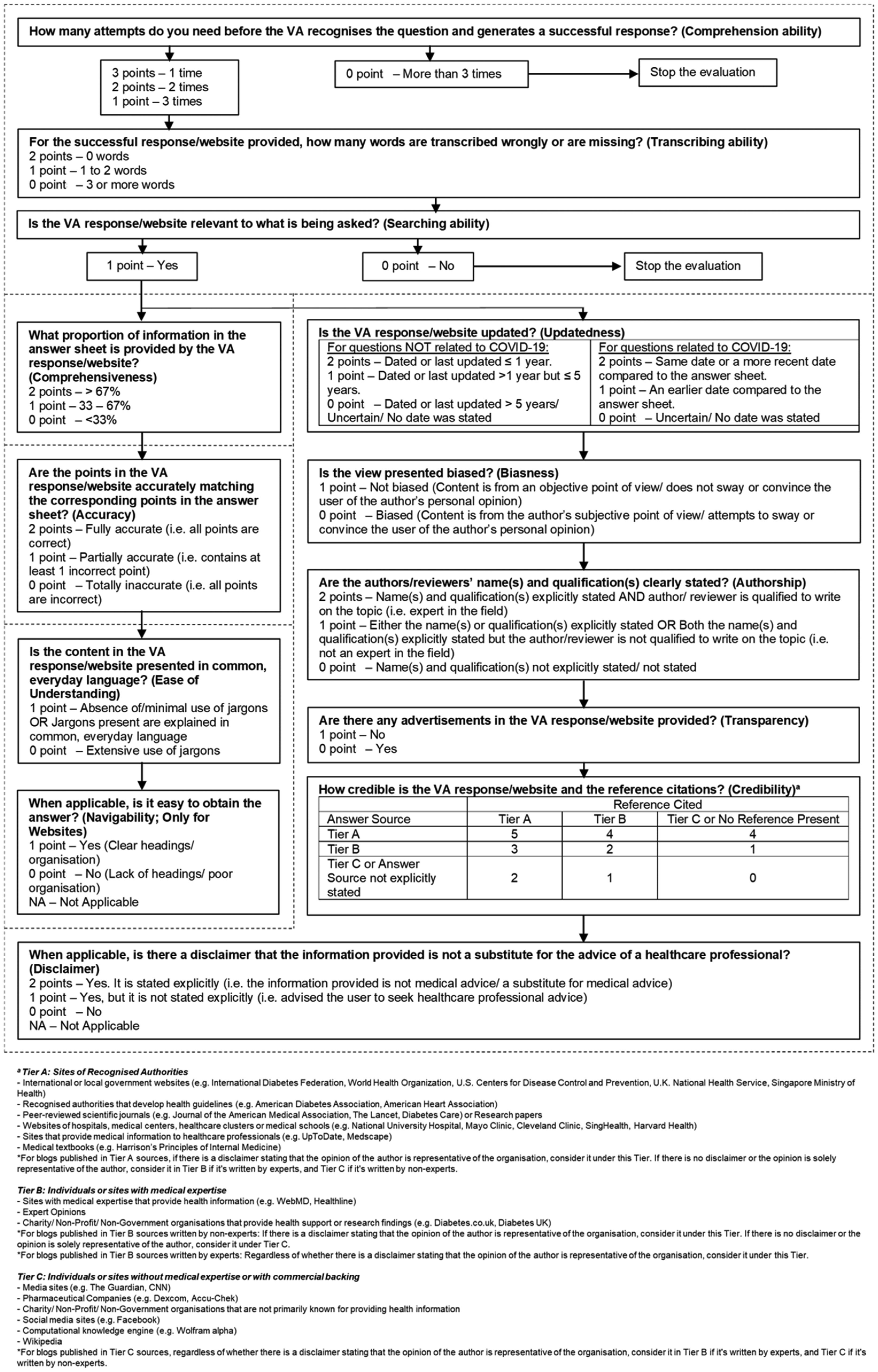
Seventy-four questions were posed to smartphone (Apple Siri, Google Assistant, Samsung Bixby) and non-smartphone DVAs (Amazon Alexa, Sulli the Diabetes Guru, Google Nest Mini, Microsoft Cortana), and their responses were compared to that of Internet Google Search. Questions were categorized under diagnosis, screening, management, treatment and complications of diabetes, and the impacts of COVID-19 on diabetes. The DVAs were evaluated on their technical ability, user-friendliness, reliability, comprehensiveness and accuracy of their responses. Data was analyzed using the Kruskal-Wallis and Wilcoxon rank-sum tests. Intraclass correlation coefficient was used to report inter-rater reliability.
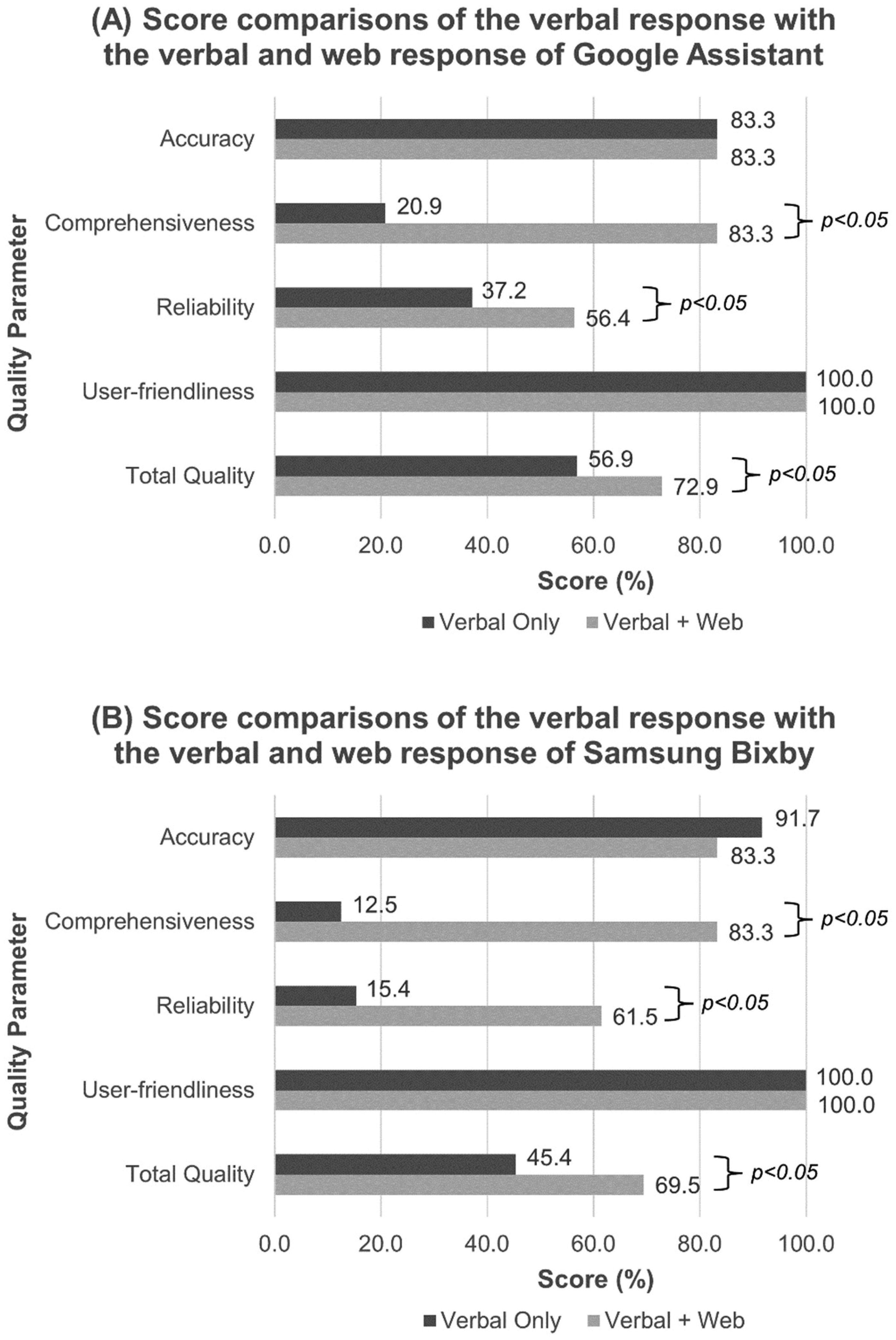
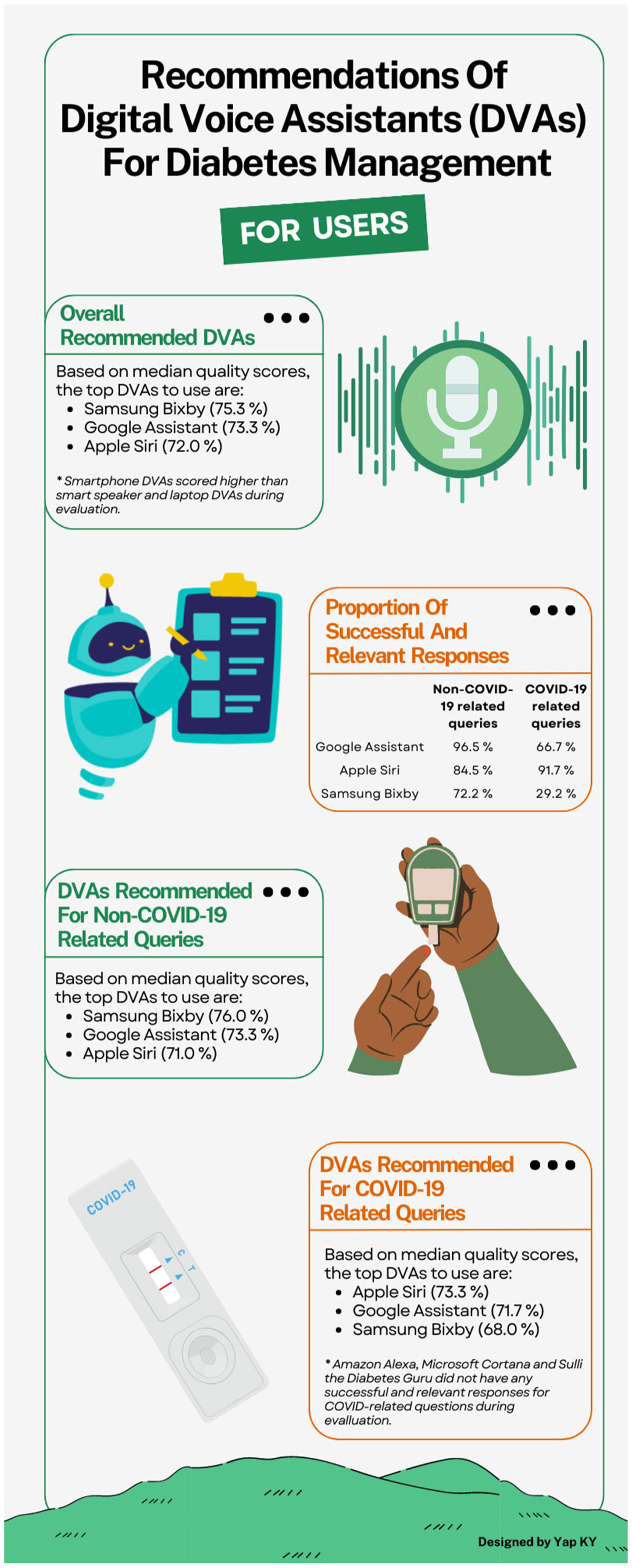
Google Assistant (n = 69/74, 93.2%), Siri and Nest Mini (n = 64/74, 86.5% each) had the highest proportions of successful and relevant responses, in contrast to Cortana (n = 23/74, 31.1%) and Sulli (n = 10/74, 13.5%), which had the lowest successful and relevant responses. Median total scores of the smartphone DVAs (Bixby 75.3%, Google Assistant 73.3%, Siri 72.0%) were comparable to that of Google Search (70.0%, p = 0.034), while median total scores of non-smartphone DVAs (Nest Mini 56.9%, Alexa 52.9%, Cortana 52.5% and Sulli the Diabetes Guru 48.6%) were significantly lower (p < 0.001). Non-smartphone DVAs had much lower median comprehensiveness (16.7% versus 100.0%, p < 0.001) and reliability scores (30.8% versus 61.5%, p < 0.001) compared to Google Search.
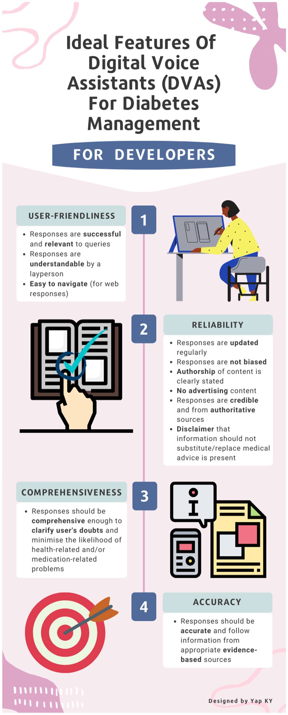
Google Assistant, Siri and Bixby were the best-performing DVAs for answering diabetes-related queries. However, the lack of successful and relevant responses by Bixby may frustrate users, especially if they have COVID-19 related queries. All DVAs scored highly for user-friendliness, but can be improved in terms of accuracy, comprehensiveness and reliability. DVA designers are encouraged to consider features related to accuracy, comprehensiveness, reliability and user-friendliness when developing their products, so as to enhance the quality of DVAs for medical purposes, such as diabetes management.
Citation: Joy Qi En Chia, Li Lian Wong, Kevin Yi-Lwern Yap. Quality evaluation of digital voice assistants for diabetes management[J]. AIMS Medical Science, 2023, 10(1): 80-106. doi: 10.3934/medsci.2023008
Digital voice assistants (DVAs) are increasingly used to search for health information. However, the quality of information provided by DVAs is not consistent across health conditions. From our knowledge, there have been no studies that evaluated the quality of DVAs in response to diabetes-related queries. The objective of this study was to evaluate the quality of DVAs in relation to queries on diabetes management.
Seventy-four questions were posed to smartphone (Apple Siri, Google Assistant, Samsung Bixby) and non-smartphone DVAs (Amazon Alexa, Sulli the Diabetes Guru, Google Nest Mini, Microsoft Cortana), and their responses were compared to that of Internet Google Search. Questions were categorized under diagnosis, screening, management, treatment and complications of diabetes, and the impacts of COVID-19 on diabetes. The DVAs were evaluated on their technical ability, user-friendliness, reliability, comprehensiveness and accuracy of their responses. Data was analyzed using the Kruskal-Wallis and Wilcoxon rank-sum tests. Intraclass correlation coefficient was used to report inter-rater reliability.
Google Assistant (n = 69/74, 93.2%), Siri and Nest Mini (n = 64/74, 86.5% each) had the highest proportions of successful and relevant responses, in contrast to Cortana (n = 23/74, 31.1%) and Sulli (n = 10/74, 13.5%), which had the lowest successful and relevant responses. Median total scores of the smartphone DVAs (Bixby 75.3%, Google Assistant 73.3%, Siri 72.0%) were comparable to that of Google Search (70.0%, p = 0.034), while median total scores of non-smartphone DVAs (Nest Mini 56.9%, Alexa 52.9%, Cortana 52.5% and Sulli the Diabetes Guru 48.6%) were significantly lower (p < 0.001). Non-smartphone DVAs had much lower median comprehensiveness (16.7% versus 100.0%, p < 0.001) and reliability scores (30.8% versus 61.5%, p < 0.001) compared to Google Search.
Google Assistant, Siri and Bixby were the best-performing DVAs for answering diabetes-related queries. However, the lack of successful and relevant responses by Bixby may frustrate users, especially if they have COVID-19 related queries. All DVAs scored highly for user-friendliness, but can be improved in terms of accuracy, comprehensiveness and reliability. DVA designers are encouraged to consider features related to accuracy, comprehensiveness, reliability and user-friendliness when developing their products, so as to enhance the quality of DVAs for medical purposes, such as diabetes management.

| [1] | Kinsella B, Mutchler A (2018) Voice assistant consumer adoption report. Voicebot.AI . Available from: https://voicebot.ai/wp-content/uploads/2018/11/voice-assistant-consumer-adoption-report-2018-voicebot.pdf. |
| [2] | National Public Media, Edison Research.The Smart Audio Report. National Public Media (2020) . Available from: https://www.nationalpublicmedia.com/insights/reports/smart-audio-report/. |
| [3] | Laricchia F (2022) Number of voice assistants in use worldwide from 2019 to 2024 (in billions). Statista . Available from: https://www.statista.com/statistics/973815/worldwide-digital-voice-assistant-in-use/. |
| [4] | Laricchia F (2022) Factors surrounding preference of voice assistants over websites and applications, worldwide, as of 2017. Statista . Available from: https://www.statista.com/statistics/801980/worldwide-preference-voice-assistant-websites-app/. |
| [5] | Kinsella B, Mutchler A (2019) Voice assistant consumer adoption in healthcare. Voicebot.AI . Available from: https://voicebot.ai/wp-content/uploads/2019/10/voice_assistant_consumer_adoption_in_healthcare_report_voicebot.pdf. |
| [6] |
Ferrand J, Hockensmith R, Houghton RF, et al. (2020) Evaluating smart assistant responses for accuracy and misinformation regarding human papillomavirus vaccination: Content analysis study. J Med Internet Res 22: e19018. https://doi.org/10.2196/19018 
|
| [7] |
Alagha EC, Helbing RR (2019) Evaluating the quality of voice assistants' responses to consumer health questions about vaccines: An exploratory comparison of Alexa, Google Assistant and Siri. BMJ Health Care Inform 26: e100075. https://doi.org/10.1136/bmjhci-2019-100075
|
| [8] |
Goh ASY, Wong LL, Yap KYL (2021) Evaluation of COVID-19 information provided by digital voice assistants. Int J Digit Health 1: 3. https://doi.org/10.29337/ijdh.25
|
| [9] |
Kocaballi AB, Quiroz JC, Rezazadegan D, et al. (2020) Responses of conversational agents to health and lifestyle prompts: investigation of appropriateness and presentation structures. J Med Internet Res 22: e15823. https://doi.org/10.2196/15823
|
| [10] |
Miner AS, Milstein A, Schueller S, et al. (2016) Smartphone-based conversational agents and responses to questions about mental health, interpersonal violence, and physical health. JAMA Intern Med 176: 619-625. https://doi.org/10.1001/jamainternmed.2016.0400
|
| [11] |
Bickmore TW, Trinh H, Olafsson S, et al. (2018) Patient and consumer safety risks when using conversational assistants for medical information: An observational study of Siri, Alexa, and Google Assistant. J Med Internet Res 20: e11510. https://doi.org/10.2196/11510
|
| [12] |
Bérubé C, Schachner T, Keller R, et al. (2021) Voice-based conversational agents for the prevention and management of chronic and mental health conditions: Systematic literature review. J Med Internet Res 23: e25933. https://doi.org/10.2196/25933
|
| [13] | World Health Organization.Global report on diabetes. World Health Organization (2016) . Available from: https://www.who.int/publications/i/item/9789241565257. |
| [14] | World Health Organization.New WHO Global Compact to speed up action to tackle diabetes. World Health Organization (2021) . Available from: https://www.who.int/news/item/14-04-2021-new-who-global-compact-to-speed-up-action-to-tackle-diabetes. |
| [15] |
Ow Yong LM, Koe LWP (2021) War on diabetes in Singapore: A policy analysis. Health Res Policy Syst 19: 15. https://doi.org/10.1186/s12961-021-00678-1
|
| [16] | Amazon. Alexa developer document—Design your skill. Amazon, (n.d.). Available from: https://developer.amazon.com/en-US/docs/alexa/design/design-your-skill.html. |
| [17] | Google DevelopersIntegrate with Google Assistant. Google, (n.d.). Available from: https://developers.google.com/assistant. |
| [18] | Martineau P (2019) Alexa, What's my blood-sugar level?. Wired . Available from: https://www.wired.com/story/alexa-whats-my-blood-sugar-level/. |
| [19] | One DropAlexa skills: One Drop. Amazon, (n.d.). Available from: https://www.amazon.com/One-Drop/dp/B072QDCSQH. |
| [20] | DataMysticAlexa skills: My Sugar by Jade Diabetes. Amazon, (n.d.). Available from: https://www.amazon.com/My-Sugar-by-Jade-Diabetes/dp/B0874717X2/ref=sr_1_3?dchild=1&keywords=diabetes&qid=1627894652&s=digital-skills&sr=1-3. |
| [21] | Epad IncGoogle Assistant: Diabetes Tips. Google, (n.d.). Available from: https://assistant.google.com/services/a/uid/00000063a0945bf1?hl=en-US. |
| [22] | Epad InccGoogle Assistant: Diabetes Checkup. Google, (n.d.). Available from: https://assistant.google.com/services/a/uid/000000e2388921d2?hl=en-US. |
| [23] | DietLabsGoogle Assistant: Well With Diabetes. Google, (n.d.). Available from: https://assistant.google.com/services/a/uid/0000000a181531b7?hl=en-US. |
| [24] | RocheAlexa skills: Sulli the Diabetes Guru. Amazon, (n.d.). Available from: https://www.amazon.com/Roche-Sulli-the-Diabetes-Guru/dp/B08BLTFY75. |
| [25] | eHealth Support NetworksAlexa skills: My Diabetes Lifestyle. Amazon, (n.d.). Available from: https://www.amazon.com/eHealth-Support-Networks-Diabetes-Lifestyle/dp/B08V8DGL69/ref=sr_1_1?dchild=1&keywords=diabetes&qid=1625367230&s=digital-skills&sr=1-1. |
| [26] | Heifner M Sulli The Diabetes Guru: Your diabetes voice assistant (2020). Available from: https://beyondtype2.org/sulli-the-diabetes-guru/. |
| [27] |
Schachner T, Keller R, Wangenheim FV (2020) Artificial intelligence-based conversational agents for chronic conditions: Systematic literature review. J Med Internet Res 22: e20701. https://doi.org/10.2196/20701
|
| [28] |
Sezgin E, Militello LK, Huang Y, et al. (2020) A scoping review of patient-facing, behavioral health interventions with voice assistant technology targeting self-management and healthy lifestyle behaviors. Transl Behav Med 10: 606-628. https://doi.org/10.1093/tbm/ibz141
|
| [29] | Cheng A, Raghavaraju V, Kanugo J, et al. (2018) Development and evaluation of a healthy coping voice interface application using the Google home for elderly patients with type 2 diabetes. 2018—15th IEEE Annual Consumer Communications and Networking Conference (CCNC) . https://doi.org/10.1109/CCNC.2018.8319283 |
| [30] |
Akturk HK, Snell-Bergeon JK, Shah VN (2021) Continuous glucose monitor with Siri integration improves glycemic control in legally blind patients with diabetes. Diabetes Technol Ther 23: 81-83. https://doi.org/10.1089/dia.2020.0320
|
| [31] | Maharjan B, Li J, Kong J, et al. (2019) Alexa, what should I eat?: A personalized virtual nutrition coach for native American diabetes patients using Amazon's smart speaker technology. 2019—IEEE International Conference on E-Health Networking, Application and Services, (HealthCom) . https://doi.org/10.1109/HealthCom46333.2019.9009613 |
| [32] | Statista Research Department.Worldwide desktop market share of leading search engines from January 2010 to July 2022. Statista (2022) . Available from: https://www.statista.com/statistics/216573/worldwide-market-share-of-search-engines/. |
| [33] |
Yap KYL, Raaj S, Chan A (2010) OncoRx-IQ: A tool for quality assessment of online anticancer drug interactions. Int J Qual Health Care 22: 93-106. https://doi.org/10.1093/intqhc/mzq004
|
| [34] | Health On The Net (HON) Foundation.HONcode certification. Health On The Net (2020) . Available from: https://myhon.ch/en/certification.html. |
| [35] | Charnock D (1998) The DISCERN Handbook: Quality criteria for consumer health information on treatment choices. Abingdon, Oxon: Radcliffe Medical Press 55 pp. Available from: https://a-f-r.org/wp-content/uploads/sites/3/2016/01/1998-Radcliffe-Medical-Press-Quality-criteria-for-consumer-health-information-on-treatment-choices.pdf. |
| [36] |
Charnock D, Shepperd S, Needham G, et al. (1999) DISCERN: An instrument for judging the quality of written consumer health information on treatment choices. J Epidemiol Community Health 53: 105-111. https://doi.org/10.1136/jech.53.2.105
|
| [37] |
Robillard JM, Jun JH, Lai JA, et al. (2018) The QUEST for quality online health information: validation of a short quantitative tool. BMC Med Inform Decis Mak 18: 87. https://doi.org/10.1186/s12911-018-0668-9
|
| [38] |
Shoemaker SJ, Wolf MS, Brach C (2014) Development of the Patient Education Materials Assessment Tool (PEMAT): A new measure of understandability and actionability for print and audiovisual patient information. Patient Educ Couns 96: 395-403. https://doi.org/10.1016/j.pec.2014.05.027
|
| [39] | Shoemaker SJ, Wolf MS, Brach C The Patient Education Materials Assessment Tool (PEMAT) and User's Guide (2013). Available from: https://www.ahrq.gov/health-literacy/patient-education/pemat.html |
| [40] | National Library of Medicine.Evaluating Internet Health Information Tutorial. MedlinePlus (2020) . Available from: https://medlineplus.gov/webeval/intro1.html. |
| [41] | Tan RY, Pua AE, Wong LL, et al. (2021) Assessing the quality of COVID-19 vaccine videos on video-sharing platforms. Explor Res Clin Soc Pharm 2: 100035. https://doi.org/10.1016/j.rcsop.2021.100035 |
| [42] | Ministry of Health Singapore.Your Diabetes Questions Answered. HealthHub (2020) . Available from: https://www.healthhub.sg/live-healthy/1392/your-diabetes-questions-answered. |
| [43] | American Diabetes Association.Frequently Asked Questions: COVID-19 and Diabetes—How COVID-19 impacts people with diabetes. American Diabetes Association . Available from: https://www.diabetes.org/coronavirus-covid-19/how-coronavirus-impacts-people-with-diabetes. |
| [44] | GoogleFAQ about Google Trends data—Trends Help. Available from: https://support.google.com/trends/answer/4365533?hl=en&ref_topic=6248052. |
| [45] | AnswerThePublicSearch listening tool for market, customer & content research. Available from: https://answerthepublic.com/. |
| [46] | American Diabetes AssociationAmerican Diabetes Association—Connected for Life. Available from: https://diabetes.org/. |
| [47] | Centers for Disease Control and Prevention.Diabetes. Centers for Disease Control and Prevention (2021) . Available from: https://www.cdc.gov/diabetes/index.html. |
| [48] | National Institute of Diabetes and Digestive and Kidney Diseases.Diabetes. National Institute of Diabetes and Digestive and Kidney diseases (NIDDK) . Available from: https://www.niddk.nih.gov/health-information/diabetes. |
| [49] | Cleveland Clinic.Diabetes: An overview. Cleveland Clinic (2021) . Available from: https://my.clevelandclinic.org/health/diseases/7104-diabetes-mellitus-an-overview. |
| [50] | US Food and Drug Administration.Food and Drug Administration homepage. US FDA . Available from: https://www.fda.gov/. |
| [51] | Diabetes UK.Diabetes UK—Know diabetes. Fight diabetes. Diabetes UK . Available from: https://www.diabetes.org.uk/. |
| [52] | UK National Health Service.Diabetes—NHS. National Health Service . Available from: https://www.nhs.uk/conditions/diabetes/. |
| [53] | Victoria State GovernmentBetter Health Channel—Diabetes. Available from: https://www.betterhealth.vic.gov.au/health/conditionsandtreatments/diabetes. |
| [54] | Diabetes AustraliaDiabetes Australia homepage. Available from: https://www.diabetesaustralia.com.au/. |
| [55] | Ministry of Health SingaporeHealthHub Health Services. Available from: https://www.healthhub.sg/. |
| [56] | National University Health System.National University Hospital: Home. National University Hospital . Available from: https://www.nuh.com.sg/Pages/Home.aspx. |
| [57] | Royal Australian College of General Practitioners, Diabetes Australia.Management of type 2 diabetes: A handbook for general practice. Royal Australian College of General Practitioners (2020) . Available from: https://www.diabetesaustralia.com.au/wp-content/uploads/Available-here.pdf. |
| [58] | Ministry of Health Singapore.Diabetes Mellitus—MOH Clinical Practice Guidelines 1/2014. Ministry of Health (2014) . Available from: https://www.moh.gov.sg/docs/librariesprovider4/guidelines/cpg_diabetes-mellitus-booklet---jul-2014.pdf. |
| [59] | Diabetes Care.Introduction: Standards of Medical Care in Diabetes—2021. Diabetes Care (2021) . Available from: https://care.diabetesjournals.org/content/44/Supplement_1. |
| [60] | National Institute for Health and Care Excellence.Type 1 diabetes in adults: Diagnosis and management—NICE guideline. National Institute for Health and Care Excellence (2021) . Available from: https://www.nice.org.uk/guidance/ng17. |
| [61] |
Cosentino F, Grant PJ, Aboyans V, et al. (2020) 2019 ESC Guidelines on diabetes, pre-diabetes, and cardiovascular diseases developed in collaboration with the EASD: The Task Force for diabetes, pre-diabetes, and cardiovascular diseases of the European Society of Cardiology (ESC) and the European Association for the Study of Diabetes (EASD). Eur Heart J 41: 255-323. https://doi.org/10.1093/eurheartj/ehz486
|
| [62] | American Diabetes Association.6. Glycemic targets: Standards of medical care in diabetes—2021. Diabetes Care (2021) 44: S73-S84. https://doi.org/10.2337/dc21-S006 |
| [63] | American Diabetes Association.Myths about Diabetes. American Diabetes Association . Available from: https://www.diabetes.org/diabetes-risk/prediabetes/myths-about-diabetes. |
| [64] | Centers for Disease Control and Prevention.Flu & people with diabetes. Centers for Disease Control and Prevention (2022) . Available from: https://www.cdc.gov/flu/highrisk/diabetes.htm. |
| [65] | Rahmatizadeh S, Valizadeh-Haghi S (2018) Evaluating the trustworthiness of consumer-oriented health websites on diabetes. Libr Philos Pract, 1786. |
| [66] |
Keselman A, Arnott Smith C, Murcko AC, et al. (2019) Evaluating the quality of health information in a changing digital ecosystem. J Med Internet Res 21: e11129. https://doi.org/10.2196/11129
|
| [67] | National Library of MedicineMedlinePlus evaluating internet health information: A tutorial National Library of Medicine (2018). Available from: https://medlineplus.gov/webeval/EvaluatingInternetHealthInformationTutorial.pdf. |
| [68] |
Smith DA (2020) Situating Wikipedia as a health information resource in various contexts: A scoping review. PLoS One 15: e0228786. https://doi.org/10.1371/journal.pone.0228786
|
| [69] | Google Developers.Policies for actions on Google. Google Developers . Available from: https://developers.google.com/assistant/console/policies/general-policies. |
| [70] | Amazon.com Inc.Alexa developer documentation: Policy requirements. Amazon . Available from: https://developer.amazon.com/en-US/docs/alexa/custom-skills/policy-testing-for-an-alexa-skill.html. |
| [71] |
Savitha S, Hirsch IB (2014) Personalized diabetes management: Moving from algorithmic to individualized therapy. Diabetes Spectrum 27: 87-91. https://doi.org/10.2337/diaspect.27.2.87
|
| [72] | Patel N 6 timely SEO strategies and resources for voice search. Available from: https://neilpatel.com/blog/seo-for-voice-search/. |
| [73] |
Shafiee G, Mohajeri-Tehrani M, Pajouhi M, et al. (2012) The importance of hypoglycemia in diabetic patients. J Diabetes Metab Disord 11: 17. https://doi.org/10.1186/2251-6581-11-17
|
| [74] | Diabetes.co.uk.Hypoglycemia (low blood glucose levels). Diabetes.co.uk (2022) . Available from: https://www.diabetes.co.uk/Diabetes-and-Hypoglycaemia.html#:~:text=Diabetes%20UK%20recommend%20that%20you,a%20non%2Ddiet%20soft%20drink. |
| [75] | Centers for Disease Control and Prevention.How to treat low blood sugar (Hypoglycemia). Centers for Disease Control and Prevention (2021) . Available from: https://www.cdc.gov/diabetes/basics/low-blood-sugar-treatment.html. |
| [76] | Amazon.com Inc.What is natural language understanding?. Amazon . Available from: https://developer.amazon.com/en-US/alexa/alexa-skills-kit/nlu. |
| [77] | Kinsella B (2019) Voice assistant demographic data—Young consumers more likely to own smart speakers while over 60 bias toward Alexa and Siri. Voicebot.ai . Available from: https://voicebot.ai/2019/06/21/voice-assistant-demographic-data-young-consumers-more-likely-to-own-smart-speakers-while-over-60-bias-toward-alexa-and-siri/. |
| [78] | Cherney K, Wood K (2022) Age of onset for type 2 diabetes: Know your risk. Healthline . Available from: https://www.healthline.com/health/type-2-diabetes-age-of-onset#age-at-diagnosis. |
 medsci-10-01-008-s001.pdf medsci-10-01-008-s001.pdf |
 |
Figures(4) / Tables(5)

Joy Qi En Chia, Li Lian Wong, Kevin Yi-Lwern Yap. Quality evaluation of digital voice assistants for diabetes management[J]. AIMS Medical Science, 2023, 10(1): 80-106. doi: 10.3934/medsci.2023008


 DownLoad: