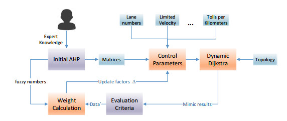
Concerning decisions for modern public transportation project, the lack of consensus between stakeholders and foreseeability of future transportation requirements might cause poor sustainability of the project. Unfortunately, many decision models give decision opinions without the test of the sustainability. Therefore, a dynamical Dijkstra simulation model is proposed to simulate the real traffic flows. In the model, the cost of the road connections is dynamically updated according to the change of the passenger flows. Then a combined decision support model using fuzzy AHP and dynamical Dijkstra simulation tests is designed. The combined model is capable of analyzing and creating consensus among different stakeholder participants in a transport development problem. The application of FAHP and dynamical Dijkstra ensures that the consensus creation is not only based on the FAHP decision making process but also on the response of the simulated execution of the decisions by dynamical Dijkstra. Thus, the decision makers by FAHP can firstly make their initial preferences in transportation planning, given the pairwise comparison matrices and generate the related weight for the traffic control parameters. And the dynamical Dijkstra simulations test the plan's setting and gives a response to iteratively adjust the FAHP matrices and parameters. The combined model is tested in different scenarios. And the results show that by the application of the proposed model, decision-makers can be more aware of the conflicts of interests among the involved groups, and they can pay more attention to possible violations causing by the change of traffic environment, including the citizen numbers, the construction cost, the roll cost, and etc., to get a more sustainable plan.
Citation: Xinlei Ma, Wen Chen, Zhan Gao, Tao Yang. Adaptive decision support model for sustainable transport system using fuzzy AHP and dynamical Dijkstra simulations[J]. Mathematical Biosciences and Engineering, 2022, 19(10): 9895-9914. doi: 10.3934/mbe.2022461
Concerning decisions for modern public transportation project, the lack of consensus between stakeholders and foreseeability of future transportation requirements might cause poor sustainability of the project. Unfortunately, many decision models give decision opinions without the test of the sustainability. Therefore, a dynamical Dijkstra simulation model is proposed to simulate the real traffic flows. In the model, the cost of the road connections is dynamically updated according to the change of the passenger flows. Then a combined decision support model using fuzzy AHP and dynamical Dijkstra simulation tests is designed. The combined model is capable of analyzing and creating consensus among different stakeholder participants in a transport development problem. The application of FAHP and dynamical Dijkstra ensures that the consensus creation is not only based on the FAHP decision making process but also on the response of the simulated execution of the decisions by dynamical Dijkstra. Thus, the decision makers by FAHP can firstly make their initial preferences in transportation planning, given the pairwise comparison matrices and generate the related weight for the traffic control parameters. And the dynamical Dijkstra simulations test the plan's setting and gives a response to iteratively adjust the FAHP matrices and parameters. The combined model is tested in different scenarios. And the results show that by the application of the proposed model, decision-makers can be more aware of the conflicts of interests among the involved groups, and they can pay more attention to possible violations causing by the change of traffic environment, including the citizen numbers, the construction cost, the roll cost, and etc., to get a more sustainable plan.

| [1] |
A. A. Rassafi, M. Vaziri, Sustainable transport indicators: definition and integration, Int. J. Environ. Sci. Technol., 2 (2005), 83–96. https://doi.org/10.1007/BF03325861 doi: 10.1007/BF03325861

|
| [2] |
T. A. Shiau, Evaluating transport infrastructure decisions under uncertainty, Transp. Plann. Technol., 37 (2014), 525–538. http://dx.doi.org/10.1080/03081060.2014.921405 doi: 10.1080/03081060.2014.921405
|
| [3] | K. Zhou, X. Peng, Z. Guo, Evaluation method of coupling between urban spatial structure and public transport system, in 2019 5th International Conference on Transportation Information and Safety (ICTIS), (2019), 723–729. http://dx.doi.org/10.1109/ICTIS.2019.8883745 |
| [4] |
M. Das, A. Roy, S. Maity, S. Kar, S. Sengupta, Solving fuzzy dynamic ship routing and scheduling problem through new genetic algorithm, Decis. Making: Appl. Manage. Eng., 2021. https://doi.org/10.31181/dmame181221030d doi: 10.31181/dmame181221030d
|
| [5] |
Ö. N. Çam, H. K. Sezen, The formulation of a linear programming model for the vehicle routing problem in order to minimize idle time, Decis. Making: Appl. Manage. Eng., 3 (2020), 22–29. https://doi.org/10.31181/dmame2003132h doi: 10.31181/dmame2003132h
|
| [6] | O. Aslan, A. Yazici, Conflict-free route planning for autonomous transport vehicle, in 2020 28th Signal Processing and Communications Applications Conference (SIU), (2020), 1–4. https://doi.org/10.1109/SIU49456.2020.9302504 |
| [7] | O. Surnin, A. Ivaschenko, P. Sitnikov, A. Suprun, A. Stolbova, O. Golovnin, Urban public transport digital planning based on an intelligent transportation system, in 2019 25th Conference of Open Innovations Association (FRUCT), (2019), 292–298. https://doi.org/10.23919/FRUCT48121.2019.8981507 |
| [8] | I. Estalayo, E. Osaba, I. Laña, J. D. Ser, Deep recurrent neural networks and optimization meta-heuristics for green urban route planning with dynamic traffic estimates, in 2019 IEEE Intelligent Transportation Systems Conference (ITSC), (2019), 1336–1342. https://doi.org/10.1109/ITSC.2019.8916957 |
| [9] |
S. Duleba, S. Moslem, Sustainable Urban transport development with stakeholder participation, an AHP-Kendall model: A case study for Mersin, Sustainability, 10 (2018), 36–47. http://doi.org/10.3390/su10103647 doi: 10.3390/su10103647
|
| [10] |
S. Duleba, S. Moslem, Examining Pareto optimality in analytic hierarchy process on real data: An application in public transport service development, Expert Syst., 116 (2019), 21–30. https://doi.org/10.1016/j.eswa.2018.08.049 doi: 10.1016/j.eswa.2018.08.049
|
| [11] |
M. Balaji, S. Santhanakrishnan, S. N. Dinesh, An application of analytic hierarchy process in vehicle routing problem, Period. Polytech. Transp. Eng., 47 (2019), 196–205. http://doi.org/10.3311/PPtr.10701 doi: 10.3311/PPtr.10701
|
| [12] |
S. Duleba, An AHP-ISM approach for considering public preferences in a public transport development decision, Transport, 6 (2019), 1–10. http://doi.org/10.3846/transport.2019.9080 doi: 10.3846/transport.2019.9080
|
| [13] |
H. Upadhyay, S. Juneja, A. Juneja, G. Dhiman, S. Kautish, Evaluation of ergonomics-related disorders in online education using fuzzy AHP, Comput. Intell. Neurosci., 2021 (2021), 1–11. https://doi.org/10.1155/2021/2214971 doi: 10.1155/2021/2214971
|
| [14] | O. Ghorbanzadeh, B. Feizizadeh, T. Blaschke, R. Khosravi, Spatially explicit sensitivity and uncertainty analysis for the landslide risk assessment of the gas pipeline networks, in Proceedings of the 21st AGILE conference on Geo-information science, (2018), 12–15. |
| [15] |
M. M. De Brito, M. Evers, A. D. S. Almoradie, Participatory flood vulnerability assessment: A multi-criteria approach, Hydrol. Earth Syst. Sci., 22 (2018), 373–390. http://doi.org/10.5194/hess-22-373-2018 doi: 10.5194/hess-22-373-2018
|
| [16] |
H. Jin, M. Zhang, Y. Yuan, Analytic network process-based multi-criteria decision approach and sensitivity analysis for temporary facility layout planning in construction projects, Appl. Sci., 8 (2018), 24–34. https://doi.org/10.3390/app8122434 doi: 10.3390/app8122434
|
| [17] |
M. Hervás-Peralta, S. Poveda-Reyes, G. D. Molero, F. E. Santarremigia, J. P. Pastor-Ferrando, Improving the performance of dry and maritime ports by increasing knowledge about the most relevant functionalities of the terminal operating system (TOS), Sustainability, 11 (2019), 1–23. https://doi.org/10.3390/su11061648 doi: 10.3390/su11061648
|
| [18] |
O. Ghorbanzadeh, B. Feizizadeh, T. Blaschke, Multi-criteria risk evaluation by integrating an analytical network process approach into GIS-based sensitivity and uncertainty analyses, Geomat. Nat. Hazards Risk, 9 (2018), 127–151. https://doi.org/10.1080/19475705.2017.1413012 doi: 10.1080/19475705.2017.1413012
|
| [19] |
S. R. Meena, O. Ghorbanzadeh, T. Blaschke, A comparative study of statistics-based landslide susceptibility models: A case study of the region affected by the Gorkha earthquake in Nepal, ISPRS Int. J. Geo-Inf., 8 (2019). https://doi.org/10.3390/ijgi8020094 doi: 10.3390/ijgi8020094
|
| [20] |
A. Hawbani, E. Torbosh, X. Wang, P. Sincak, L. Zhao, A. Al-Dubai, Fuzzy-based distributed protocol for vehicle-to-vehicle communication, IEEE Trans. Fuzzy Syst., 29 (2021), 612–626. https://doi.org/10.1109/TFUZZ.2019.2957254 doi: 10.1109/TFUZZ.2019.2957254
|
| [21] |
S. Moslem, O. Ghorbanzadeh, T. Blaschke, S. Duleba, Analysing stakeholder consensus for a sustainable transport development decision by the fuzzy AHP and interval AHP, Sustainability, 11 (2019), 1–22. http://doi.org/10.3390/su11123271 doi: 10.3390/su11123271
|
| [22] |
V. Mohagheghi, S. M. Mousavi, M. Aghamohagheghi, B. Vahdani, A new approach of multi-criteria analysis for the evaluation and selection of sustainable transport investment projects under uncertainty: A case study, Int. J. Comput. Intell. Syst., 10 (2017), 605–626. https://doi.org/10.2991/ijcis.2017.10.1.41 doi: 10.2991/ijcis.2017.10.1.41
|
| [23] |
P. Ziemba, Selection of electric vehicles for the needs of sustainable transport under conditions of uncertainty—a comparative study on fuzzy MCDA Methods, Energies, 14 (2021), 7786. https://doi.org/10.3390/en14227786 doi: 10.3390/en14227786
|
| [24] |
B. Buran, M. Erçek, Public transportation business model evaluation with Spherical and Intuitionistic Fuzzy AHP and sensitivity analysis, Expert Syst. Appl., 204 (2022), 117519. https://doi.org/10.1016/j.eswa.2022.117519 doi: 10.1016/j.eswa.2022.117519
|
| [25] |
J. Wątróbski, K. Małecki, K. Kijewska, S. Iwan, A. Karczmarczyk, R. G. Thompson, Multi-criteria analysis of electric vans for city logistics, Sustainability, 9 (2017), 1453. https://doi.org/10.3390/su9081453 doi: 10.3390/su9081453
|
| [26] |
M. H. Ha, Z. Yang, M. W. Heo, A new hybrid decision making framework for prioritising port performance improvement strategies, Asian J. Shipp. Logist., 33 (2017), 105–116. https://doi.org/10.1016/j.ajsl.2017.09.001 doi: 10.1016/j.ajsl.2017.09.001
|
| [27] |
M. Yavuz, B. Oztaysi, S. C. Onar, C. Kahraman, Multi-criteria evaluation of alternative fuel vehicles via a hierarchical hesitant fuzzy linguistic model, Expert Syst., 42 (2015), 2835–2848. https://doi.org/10.1016/j.eswa.2014.11.010 doi: 10.1016/j.eswa.2014.11.010
|
| [28] |
U. R. Tuzkaya, Evaluating the environmental effects of transportation modes using an integrated methodology and an application, Int. J. Environ. Sci. Tech., 6 (2009), 277–290. http://doi.org/10.1007/BF03327632 doi: 10.1007/BF03327632
|
| [29] |
A. Awasthi, S. SChauhan, A hybrid approach integrating Affinity Diagram, AHP and fuzzy TOPSIS for sustainable city logistics planning, Appl. Math. Modell., 36 (2012), 573–584. https://doi.org/10.1016/j.apm.2011.07.033 doi: 10.1016/j.apm.2011.07.033
|
| [30] |
W. Pedrycz, Analytic hierarchy process (AHP) in group decision making and its optimization with an allocation of information granularity, IEEE Trans. Fuzzy Syst., 19 (2011), 527–539. https://doi.org/10.1109/TFUZZ.2011.2116029 doi: 10.1109/TFUZZ.2011.2116029
|
| [31] |
T. T. Nguyen, L. Gordon-Brown, Constrained fuzzy hierarchical analysis for portfolio selection under higher moments, IEEE Trans. Fuzzy Syst., 20 (2012), 666–682. https://doi.org/10.1109/TFUZZ.2011.2181520 doi: 10.1109/TFUZZ.2011.2181520
|
| [32] |
K. T. T. Bui, D. T. Bui, J. Zou, C. Van Doan, I. Revhaug, A novel hybrid artificial intelligent approach based on neural fuzzy inference model and particle swarm optimization for horizontal displacement modeling of hydropower dam, Neural Comput., 29 (2018), 1495–1506. https://doi.org/10.1007/s00521-016-2666-0 doi: 10.1007/s00521-016-2666-0
|
Figures(11) / Tables(2)

Xinlei Ma, Wen Chen, Zhan Gao, Tao Yang. Adaptive decision support model for sustainable transport system using fuzzy AHP and dynamical Dijkstra simulations[J]. Mathematical Biosciences and Engineering, 2022, 19(10): 9895-9914. doi: 10.3934/mbe.2022461


 DownLoad: