


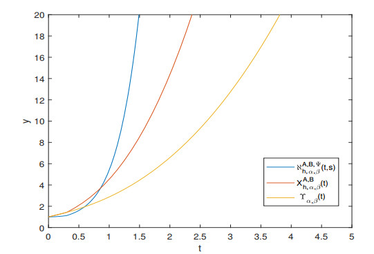
Figure 1.
Comparison of functions ℵA,B,Ψh,α,β(t,s), XA,Bh,α,β(t), and Υα,β(t) for α=0.9, β=1, h=0.3, A=1, B=1, s=0, Ψ(t)=t2.
We give a representation of solutions to linear nonhomogeneous Ψ-fractional delayed differential equations with noncommutative matrices. We newly define Ψ-delay perturbation of Mittag-Leffler type matrix function with two parameters and apply the method of variation of constants to obtain the representation of the solutions. We investigate the existence and uniqueness of solutions for a class of Ψ-fractional delayed semilinear differential equations by using Banach Fixed Point Theorem. Further, we establish the Ulam-Hyers stability result for the analyzed problem. Finally, we provide some examples to illustrate the applicability of our results.
Citation: Mustafa Aydin, Nazim I. Mahmudov, Hüseyin Aktuğlu, Erdem Baytunç, Mehmet S. Atamert. On a study of the representation of solutions of a Ψ-Caputo fractional differential equations with a single delay[J]. Electronic Research Archive, 2022, 30(3): 1016-1034. doi: 10.3934/era.2022053
| [1] | Peng Gao, Pengyu Chen . Blowup and MLUH stability of time-space fractional reaction-diffusion equations. Electronic Research Archive, 2022, 30(9): 3351-3361. doi: 10.3934/era.2022170 |
| [2] | Nelson Vieira, M. Manuela Rodrigues, Milton Ferreira . Time-fractional telegraph equation of distributed order in higher dimensions with Hilfer fractional derivatives. Electronic Research Archive, 2022, 30(10): 3595-3631. doi: 10.3934/era.2022184 |
| [3] | Vo Van Au, Jagdev Singh, Anh Tuan Nguyen . Well-posedness results and blow-up for a semi-linear time fractional diffusion equation with variable coefficients. Electronic Research Archive, 2021, 29(6): 3581-3607. doi: 10.3934/era.2021052 |
| [4] | E. A. Abdel-Rehim . The time evolution of the large exponential and power population growth and their relation to the discrete linear birth-death process. Electronic Research Archive, 2022, 30(7): 2487-2509. doi: 10.3934/era.2022127 |
| [5] | Li Tian, Ziqiang Wang, Junying Cao . A high-order numerical scheme for right Caputo fractional differential equations with uniform accuracy. Electronic Research Archive, 2022, 30(10): 3825-3854. doi: 10.3934/era.2022195 |
| [6] | Anh Tuan Nguyen, Chao Yang . On a time-space fractional diffusion equation with a semilinear source of exponential type. Electronic Research Archive, 2022, 30(4): 1354-1373. doi: 10.3934/era.2022071 |
| [7] | Akeel A. AL-saedi, Jalil Rashidinia . Application of the B-spline Galerkin approach for approximating the time-fractional Burger's equation. Electronic Research Archive, 2023, 31(7): 4248-4265. doi: 10.3934/era.2023216 |
| [8] | Minzhi Wei . Existence of traveling waves in a delayed convecting shallow water fluid model. Electronic Research Archive, 2023, 31(11): 6803-6819. doi: 10.3934/era.2023343 |
| [9] | Ziqing Yang, Ruiping Niu, Miaomiao Chen, Hongen Jia, Shengli Li . Adaptive fractional physical information neural network based on PQI scheme for solving time-fractional partial differential equations. Electronic Research Archive, 2024, 32(4): 2699-2727. doi: 10.3934/era.2024122 |
| [10] | Huifu Xia, Yunfei Peng . Pointwise Jacobson type necessary conditions for optimal control problems governed by impulsive differential systems. Electronic Research Archive, 2024, 32(3): 2075-2098. doi: 10.3934/era.2024094 |
We give a representation of solutions to linear nonhomogeneous Ψ-fractional delayed differential equations with noncommutative matrices. We newly define Ψ-delay perturbation of Mittag-Leffler type matrix function with two parameters and apply the method of variation of constants to obtain the representation of the solutions. We investigate the existence and uniqueness of solutions for a class of Ψ-fractional delayed semilinear differential equations by using Banach Fixed Point Theorem. Further, we establish the Ulam-Hyers stability result for the analyzed problem. Finally, we provide some examples to illustrate the applicability of our results.
The origins of fractional calculus may be traced back to the late seventeenth century, when Newton's and Leibniz's work provided a foundation for the development of traditional calculus. Leibniz created the notation dndtng(t) to symbolize the derivative of the function g of order n. When he conveyed this to de l'Hôpital, the second one enquired what happens if n=12. This is at the turning point for fractional calculus. The Riemann–Liouville fractional integral and derivative are the most classical fractional calculus operators [1,2]. Caputo contributed significantly by proposing a new concept of fractional derivatives that is more suited to specific physical circumstances [3,4]. Moreover, numerous other fractional operator families have been introduced and researched up to this point, out of which Prabhakar, Hadamard, Hilfer, Grünwald–Letnikov, Marchaud, and Erdélyi–Kober are just a few to mention [1,2,5,6]. Owing to the vast number of definitions related to fractional operator, it is necessary to define so certain generalized fractional operators that the traditional ones are special instances. This allows researchers to operate on a broad scale and demonstrate results that may subsequently be applied to specific circumstances by applied researchers[7]. For example, several generic classes of fractional operators were presented in [8].
The widespread usage of fractional differential equations (FDEs) in engineering, economics, physics, and other research fields inspired us to work on this topic [1,3,5,9,10,11]. There are numerous ways for solving FDEs analytically or numerically in the literature. One of the most difficult issues in the field of fractional calculus is to create some adequate methods for obtaining analytic solutions for specific kinds of FDEs numerically. Some academics have been occupied with adding fractional extensions related to well-known integral transforms like the Fourier and the Laplace transforms, in the last few years [12,13,14,15,16,17].
Over the last several decades, mathematical descriptions based on FDE linked to non-integral order derivatives have shown a highly valuable stuff for describing many phenomena such as viscoelasticity, anomalous diffusion, control and stability theory, etc. Delay (or retardation) is recognized to occur in chemical processes and many areas. The rate of evolution of these processes is generally dependent on prior history, which is a distinguishing property of the corresponding mathematical models. Differential equations are used to represent these issues and are referred to as delayed differential equations. The underlying qualitative theory about Eq (1.1), particularly in the linear case, is well understood. Time-delay of FDE, which include both delays and non-integer derivatives, allow single one of delayed differential equations. This method is valuable in technical applications for building extremely realistic simulations of specific processes and systems having memory. One can use in analysis and discussion of diverse time-delayed systems, as well as the stabilization and control of these systems via state feedback. A linear system's solution is well-known ν′(t)=Aν(t), t∈R+ has the form ν(t)=eAtν(0), where eAt is known as fundamental matrix in the literature. We note that finding a fundamental matrix associated with a delayed linear system becomes more complicated.
| ν′(t)=Aν(t)+Bν(t−h), t≥0, h>0ν(t)=η(t), −h≤t≤0 |
where A,B∈Mn×n(R). Under the statement of permutation(commutation) of matrices A and B, the authors in [18] offered an excellent solution for the system which is both delayed and homogeneous and linear by defining the exponential delay matrix eBth. In the work of [19], researchers discussed the above problem with the fractional version when A=Θ. Mahmudov in references [20,21] handled the fractional delay differential equations with the classical Caputo and Riemann-Liouville derivative and noncommutative coefficient matrices. Almeida in the study of [22] investigated Caputo type fractional derivative with reference to further function and remarkable results relevant to this derivative.
Motivated by the pioneer works of [18,19,20,22,23], we consider the following nonhomogeneous linear Ψ-Caputo fractional delay differential system
| C−h+DαΨ(x)ν(x)=Aν(x)+Bν(x−h)+f(x), 0<x≤T, h>0,ν(x)=η(x), −h≤x≤0. | (1.1) |
where C−h+DαΨ(x) is Ψ-Caputo fractional derivative, Ψ(x):R→R is increasing and Ψ′(x)≠0 for every x∈[−h,T], A and B are constant coefficient square matrices which do not have to be permutable, f∈C([0,T],Rn), and η(x)∈C1([−h,0],Rn). After obtaining a solution of the former system (1.1), we can extend it to the following system (1.2). Here is that the nonlinear Ψ-Caputo fractional delay differential system is
| C−h+DαΨ(x)ν(x)=Aν(x)+Bν(x−h)+f(x,ν(x)), 0<x≤T, h>0,ν(x)=η(x), −h≤x≤0. | (1.2) |
Each of details is as given in the system (1.1). Note that, by choosing Ψ(x)=x and Ψ(x)=lnx we observe the above differential equations reduces to Caputo fractional linear delay differential equations (see [20]) and Hadamard fractional linear delay differential equations, respectively. It should be stressed out that the Ψ-fractional derivative is defined with respect to another function and unifies several definitions of fractional derivatives available in the literature. Thus the Ψ-fractional derivative covers a wide class of fractional derivatives and provides a platform to obtain a particular one by fixing the function Ψ. The function space and the physical meaning were recently provided in [24,25].
Before finishing the introduction, we remind some notations which are valid in the rest of the paper. Let a,b∈R with a<b which is the set of all real numbers. Then Rn is the well-known Euclidean space whose dimension is n∈{1,2,3,...}. Also, let
| C([a,b],Rn)={μ:[a,b]→Rn:μ is continuous} |
with the maximum norm ‖.‖∞, which is
| ‖μ‖∞=maxt∈[a,b]‖μ(t)‖, |
where ‖.‖ is an arbitrary norm on Rn. Let AC[a,b] be the space of functions which are absolutely continuous on [a,b]. For n∈{1,2,3,...} we denote by ACn[a,b] the space of complex-valued functions f(x) which have continuous derivatives up to order n−1 on [a,b] such that f(n−1)(x)∈AC[a,b].
Definition 2.1. Let a function f and an increasing function Ψ on [a,b] be integrable and continuously differentiable, respectively and let Ψ′(t)≠0 t∈[a,b]. Ψ-Riemann-Liouville (RL) fractional integrals of f of order α>0 are given by [1]
| RLa+IαΨ(t)f(t):=1Γ(α)∫taΨ′(s)(Ψ(t)−Ψ(s))α−1f(s)ds=1Γ(α)∫ta(Ψ(t)−Ψ(s))α−1f(s)dΨ(s), |
and Ψ-RL fractional derivatives of f of order α>0 are given by
| RLa+DαΨ(t)f(t):=(1Ψ′(t)ddt)na+In−αΨ(t)f(t)=1Γ(n−α)(1Ψ′(t)ddt)n∫taΨ′(s)(Ψ(t)−Ψ(s))n−α−1f(s)ds=1Γ(n−α)(1Ψ′(t)ddt)n∫ta(Ψ(t)−Ψ(s))n−α−1f(s)dΨ(s), |
where n=[α]+1.
Definition 2.2. Let α∈R+ and n∈N [1]. If f,Ψ∈ACn([a,b],R) with Ψ is increasing and Ψ′(x)≠0 for every x∈[a,b], then the left Ψ-Caputo fractional derivative of f of order α is defined as
| Ca+DαΨ(t)f(t):=a+In−αΨ(t)(1Ψ′(t)ddt)nf(t) | (2.1) |
where n=[α]+1. Shortly, we use the abbreviation symbol as
| f[n]Ψ(t):=(1Ψ′(t)ddt)nf(t) |
Clearly,
| C−h+DαΨ(t)c=0 |
where c is a constant number.
Theorem 2.3. Let f∈ACn([a,b],R) and α∈R+ [1], then
| ( Ca+DαΨ(t)f)(t)= RLa+DαΨ(t)[f(t)−n−1∑k=0(Ψ(t)−Ψ(a))kf[k]Ψ(a)k!] |
Lemma 2.4. Let R(α)≥0 and R(β)>0 [1], then we have
| Ca+DαΨ(t)(Ψ(x)−Ψ(a))β−1(t)=Γ(β)Γ(β−α)(Ψ(t)−Ψ(a))β−α−1. |
Definition 2.5. Two parameters Mittag-Leffler type matrix function Υα,β(A,t):R→Rn×n is defined by
| Υα,β(t):=tβ−1Eα,β(Atα):=tβ−1∞∑k=0AktαkΓ(αk+β), α,β>0,t∈R |
Definition 2.6. Delayed two parameters Mittag-Leffler type matrix EBh,α,β:R→Rn is given by
| EBh,α,β(t)={Θ, −∞<t≤−hI(h+t)β−1Γ(β), −h<t≤0∑lj=0Bj(t−(j−1)h)jα+β−1Γ(jα+β), (l−1)h<t≤lh |
where l∈N+ and Θ and I are the zero and identity matrices.
Definition 2.7. The delayed perturbation of Mittag-Leffler type matrix function XA,Bh,α,β(⋅):[0,∞)→Rn generated by A,B is defined by [20]
| XA,Bh,α,β(t):={Θ,−h≤t<0,I,t=0,∞∑k=0p∑j=0Qk+1(jh)(t−jh)kα+β−1Γ(kα+β),ph<t≤(p+1)h, |
where Qk+1(jh)=AQk(jh)+BQk(jh−h), Q0(s)=Qk(−h)=Θ, Q1(0)=I for k=0,1,2,… ands=0,h,2h,… Θ and I are the zero and identity matrices.
Definition 2.8. If ∀ϵ>0 and for any solution ν∈C([0,T],Rn) of inequality
| ‖( CDαΨ(t)ν)(t)−Aν(t)−Bν(t−h)−f(t,ν(t))‖≤ϵ | (2.2) |
then there exists a solution μ∈C([0,T],Rn) of (1.2), and a uh∈R+ such that
| ‖ν(t)−μ(t)‖≤uh.ϵ | (2.3) |
∀t∈[0,T], then (1.2) is called Ulam-Hyers stable.
Remark 2.9. A function μ∈C1([0,T],Rn) is a solution of the inequality (2.2) if and only if there exist at least h∈C([0,T],Rn) satisfying
● ‖h(t)‖≤ε (ε>0),
● ( CDαΨ(t)μ)(t)=Aμ(t)+Bμ(t−h)+f(t,μ(t))+h(t).
Definition 3.1. Ψ-delay perturbation of Mittag-Leffler type matrix function with two parameters ℵA,B,Ψh,α,β:R×R→Rn is given as
| ℵA,B,Ψh,α,β(t,s)={Θ, t−s∈[−h,0)I, t=s∞∑i=0p−1∑j=0Qi+1(jh)[Ψ(t)−Ψ(s+jh)]iα+β−1Γ(iα+β), t−s∈((p−1)h,ph] | (3.1) |
where Ψ(t):R→R is an increasing function such that Ψ(0)=0 and Ψ′(t)≠0 for every t∈[−h,T], Θ and I represent the zero matrix and identity matrix, respectively. From [20], the matrices Qk(s) are defined for s=kh with k=0,1,2,... as
| Q0(s)=Θ, Q1(0)=I, Qk(−h)=Θ, Qk+1(s)=AQk(s)+BQk(s−h). |
Remark 3.2. From Eq (3.1) choosing Ψ(t)=t, the Ψ-delay perturbation of Mittag-Leffler type matrix with two parameters reduces to the traditional one which is introduced and investigated in [20].
Lemma 3.3. ℵA,B,Ψh,α,β(t,s) is jointly continuous in 0<s<t<∞.
Proof. Without loss of generality we consider the case s=0. For (p−1)h<tη<ph,p=1,2,…. Then
| limt→tηℵA,B,Ψh,α,β(t,0)=limt→tη∞∑i=0p−1∑j=0Qi+1(jh)[Ψ(t)−Ψ(jh)]iα+β−1Γ(iα+β)=∞∑i=0p−1∑j=0Qi+1(jh)limt→tη[Ψ(t)−Ψ(jh)]iα+β−1Γ(iα+β)=∞∑i=0p−1∑j=0Qi+1(jh)[Ψ(tη)−Ψ(jh)]iα+β−1Γ(iα+β)=ℵA,B,Ψh,α,β(tη,0). |
For tη=ph,p=1,2,…. Then
| limt→t−ηℵA,B,Ψh,α,β(t,0)=limt→ph−ℵA,B,Ψh,α,β(t,0)=limt→ph−(∞∑i=0Qi+1(0)[Ψ(t)]iα+β−1Γ(iα+β)+∞∑i=0Qi+1(h)[Ψ(t)−Ψ(h)]iα+β−1Γ(iα+β)+⋯+∞∑i=0Qi+1((p−1)h)[Ψ(t)−Ψ((p−1)h)]iα+β−1Γ(iα+β))=∞∑i=0Qi+1(0)[Ψ(ph)]iα+β−1Γ(iα+β)+∞∑i=0Qi+1(h)[Ψ(ph)−Ψ(h)]iα+β−1Γ(iα+β)+⋯+∞∑i=0Qi+1((p−1)h)[Ψ(ph)−Ψ((p−1)h)]iα+β−1Γ(iα+β)=ℵA,B,Ψh,α,β(ph,0)=ℵA,B,Ψh,α,β(tη,0). |
| limt→t+ηℵA,B,Ψh,α,β(t,0)=limt→ph+∞∑i=0p∑j=0Qi+1(jh)[Ψ(t)−Ψ(jh)]iα+β−1Γ(iα+β)=∞∑i=0p−1∑j=0Qi+1(jh)limt→ph+[Ψ(t)−Ψ(jh)]iα+β−1Γ(iα+β)+limt→ph+∞∑i=0Qi+1(ph)[Ψ(t)−Ψ(ph)]iα+β−1Γ(iα+β)=∞∑i=0p−1∑j=0Qi+1(jh)[Ψ(ph)−Ψ(jh)]iα+β−1Γ(iα+β)=limt→ph−ℵA,B,Ψh,α,β(t,0)=limt→t−ηℵA,B,Ψh,α,β(t,0). |
In brief, ℵA,B,Ψh,α,β(t,s) is continuous with respect to t∈(0,∞).
Now, we give an explicit solution of homogenous part of (1.1), which is f=0.
Lemma 3.4. ℵA,B,Ψh,α,1(t,s) is a solutionof
| C−h+DαΨ(t)ℵA,B,Ψh,α,1(t,s)=AℵA,B,Ψh,α,1(t,s)+BℵA,B,Ψh,α,1(t,s+h). | (3.2) |
Proof. We apply the mathematical induction method to prove that ℵA,B,Ψh,α,1(t,s) satisfy the differential Eq (3.2) for all t−s∈((p−1)h,ph]. For p=1, 0<t−s≤h, we have that
| ℵA,B,Ψh,α,1(t,s)=∞∑i=0Qi+1(0)[Ψ(t)−Ψ(s)]iαΓ(iα+1). |
From the definition, we know that Qi+1(0)=Ai. Therefore,
| ℵA,B,Ψh,α,1(t,s)=∞∑i=0Ai[Ψ(t)−Ψ(s)]iαΓ(iα+1)=Eα(A[Ψ(t)−Ψ(s)]α) |
and ℵA,B,Ψh,α,1(t,s+h)=Θ. By using these equalities, we get
| C−h+DαΨ(t)ℵA,B,Ψh,α,1(t,s)= C−h+DαΨ(t)(1+∞∑k=1Ak[Ψ(t)−Ψ(s)]kαΓ(kα+1))=∞∑k=1AkΓ((k−1)α+1)[Ψ(t)−Ψ(s)]α(k−1)=A∞∑k=0AkΓ(kα+1)[Ψ(t)−Ψ(s)]αk=AℵA,B,Ψh,α,1(t,s)+BℵA,B,Ψh,α,1(t,s+h). |
Assume that the following relation
| ℵA,B,Ψh,α,1(t,s)=∞∑k=0n−1∑m=0Qk+1(mh)[Ψ(t)−Ψ(s+mh)]kαΓ(kα+1) |
holds for p−1=n−1. Now, let p−1=n, we obtain
| C−h+DαΨ(t)ℵA,B,Ψh,α,1(t,s)=∞∑k=0n∑l=0Qk+1(lh) C−h+DαΨ[Ψ(t)−Ψ(s+lh)]kαΓ(kα+1)=∞∑k=0n∑l=0Qk+1(lh)[Ψ(t)−Ψ(s+lh)](k−1)αΓ((k−1)α+1)=∞∑k=1n∑l=0[AQk(lh)+BQk((l−1)h)][Ψ(t)−Ψ(s+lh)](k−1)αΓ((k−1)α+1)=∞∑k=1n∑l=0AQk(lh)[Ψ(t)−Ψ(s+lh)](k−1)αΓ((k−1)α+1)+∞∑k=1n∑l=1BQk((l−1)h)[Ψ(t)−Ψ(s+lh)](k−1)αΓ((k−1)α+1)=∞∑k=0n∑l=0AQk+1(lh)[Ψ(t)−Ψ(s+lh)]kαΓ(kα+1)+∞∑k=0n−1∑l=0BQk+1(lh)[Ψ(t)−Ψ(s+lh+h)]kαΓ(kα+1)=AℵA,B,Ψh,α,1(t,s)+BℵA,B,Ψh,α,1(t,s+h). |
Then, the proof is completed.
Lemma 3.5. Let t−s∈((p−1)h,ph]. We get the following equalities
(a) ∫ts+mh[Ψ(t)−Ψ(r)]−α[Ψ(r)−Ψ(s+mh)](i+1)α+1dΨ(r)=[Ψ(t)−Ψ(s+mh)]iαB(1−α,iα+α)
(b) ∫ts[Ψ(t)−Ψ(r)]−αℵA,B,Ψh,α,α(r,s)dΨ(r)=∑∞i=0∑p−1j=0Qi+1(jh)[Ψ(t)−Ψ(s+jh)]iαΓ(1−α)Γ(iα+1)
where B(.,.) is the well-known beta function.
Proof. We apply simple substitution as z=Ψ(r)−Ψ(s+mh), we get dz=dψ(r) Thus, we have
| ∫ts+mh[Ψ(t)−Ψ(r)]−α[Ψ(r)−Ψ(s+mh)](i+1)α+1dΨ(r)=∫Ψ(t)−Ψ(s+mh)0[(Ψ(t)−Ψ(s+mh)−z)]−αz(i+1)α−1dz=∫Ψ(t)−Ψ(s+mh)0[Ψ(t)−Ψ(s+mh)]−α[1−zΨ(t)−Ψ(s+mh)]−αz(i+1)α−1dz. |
Again, if we apply one more substitution as y=zΨ(t)−Ψ(s+mh), then dy=dzΨ(t)−Ψ(s+mh). Then we get,
| ∫ts+mh[Ψ(t)−Ψ(r)]−α[Ψ(r)−Ψ(s+mh)](i+1)α+1dΨ(r)=[Ψ(t)−Ψ(s+mh)]iα∫10(1−y)−αy(i+1)α−1dy=[Ψ(t)−Ψ(s+mh)]iαB(1−α,iα+α). | (3.3) |
By using the definition of ℵA,B,Ψh,α,β(t,s), we have
| ∫ts[Ψ(t)−Ψ(r)]−αℵA,B,Ψh,α,α(r,s)dΨ(r)=∫ts[Ψ(t)−Ψ(r)]−α∞∑m=0p−1∑j=0Qm+1(jh)[Ψ(r)−Ψ(s+jh)](m+1)α+1Γ((m+1)α)dΨ(r)=∞∑m=01Γ((m+1)α)p−1∑j=0Qm+1(jh)∫ts[Ψ(t)−Ψ(r)]−α[Ψ(r)−Ψ(s+jh)](m+1)α+1dΨ(r)=∞∑m=01Γ((m+1)α)Qm+1(0)∫ts[Ψ(t)−Ψ(r)]−α[Ψ(r)−Ψ(s)](m+1)α+1dΨ(r)+∞∑m=01Γ((m+1)α)Qm+1(h)∫ts+h[Ψ(t)−Ψ(r)]−α[Ψ(r)−Ψ(s+h)](m+1)α+1dΨ(r) ⋮+∞∑m=01Γ((m+1)α)Qm+1((p−1)h)×∫ts+(p−1)h[Ψ(t)−Ψ(r)]−α[Ψ(r)−Ψ(s+(p−1)h)](m+1)α+1dΨ(r). | (3.4) |
So, from Eqs (3.3) and (3.4), we get
| ∫ts[Ψ(t)−Ψ(r)]−αℵA,B,Ψh,α,α(r,s)Ψ(r)=∞∑i=01Γ((i+1)α)Qi+1(0)[Ψ(t)−Ψ(s)]iαB(1−α,iα+α)+∞∑i=01Γ((i+1)α)Qi+1(h)[Ψ(t)−Ψ(s+h)]iαB(1−α,iα+α) ⋮+∞∑i=01Γ((i+1)α)Qi+1((p−1)h)[Ψ(t)−Ψ(s+(p−1)h)]iαB(1−α,iα+α)=∞∑i=0p−1∑j=01Γ((i+1)α)Qi+1(jh)[Ψ(t)−Ψ(s+jh)]iαB(1−α,iα+α)=∞∑k=0p−1∑m=01Γ((k+1)α)Qk+1(mh)[Ψ(t)−Ψ(s+mh)]kαΓ(1−α)Γ(kα+α)Γ(kα+1)=∞∑k=0p−1∑j=0Qk+1(mh)[Ψ(t)−Ψ(s+mh)]kαΓ(1−α)Γ(kα+1). | (3.5) |
Theorem 3.6. If we consider the problem in Eq (1.1) with zero initial condition, which is ν(t)=0, t∈[−h,0], then the solution ν(t) has a form
| ν(t)=∫t−hℵA,B,Ψh,α,α(t,s)f(s)dΨ(s), t≥0. |
Proof. By variation of constants method, if ν(t) is any solution of nonhomogeneous system, then the form of ν(t) must be satisfy the following form
| ν(t)=∫t−hℵA,B,Ψh,α,α(t,s)c(s)dΨ(s), 0≤t | (3.6) |
where ν(0)=0 and c:[−h,t]→Rn, is a differentiable function which is not known. Applying the Ψ-Caputo fractional derivative in Eq (3.6), we get:
1) For p=1, we have 0≤t≤h. It is clear that t−h<0, by the zero initial condition we have ν(t−h)=0. So, according to Eq (1.1) we get
| C−h+DαΨ(t)ν(t)=Aν(t)+Bν(t−h)+f(t)=Aν(t)+f(t)=A∫t−hℵA,B,Ψh,α,α(t,s)c(s)dΨ(s)+f(t). |
On the other hand, by the assumption of zero initial condition we have ν(−h)=0. So, we get
| ( C−h+DαΨ(t)ν)(t)= RL−h+DαΨ(t)(ν(t)−ν(−h))= RL−h+DαΨ(t)(ν(t))= RL−h+DαΨ(t)(∫t−hℵA,B,Ψh,α,α(t,s)c(s)dΨ(s)). |
Now, according to Definition 2.1, we have
| ( C−h+DαΨ(t)ν)(t)=1Γ(1−α)1Ψ′(t)ddt∫t−h[Ψ(t)−Ψ(r)]−α(∫r−hℵA,B,Ψh,α,α(r,s)c(s)dΨ(s))dΨ(r)=1Γ(1−α)1Ψ′(t)∞∑i=0Aiddt∫t−hc(s)∫ts[Ψ(t)−Ψ(r)]−α([Ψ(r)−Ψ(s)]iα+α−1Γ(iα+α)dΨ(r))dΨ(s) |
If we use Lemma 3.5 (a) to inner integral, we get
| ( C−hDαΨ(t)ν)(t)=1Γ(1−α)1Ψ′(t)∞∑i=0Aiddt∫t−hc(s)(Ψ(t)−Ψ(s))iαΓ(iα+α)B(1−α,iα+α)dΨ(s)=1Ψ′(t)∞∑i=0Aiddt∫t−hc(s)(Ψ(t)−Ψ(s))iαΓ(iα+1)dΨ(s)=1Ψ′(t)ddt∫t−hc(s)dΨ(s)+1Ψ′(t)∞∑i=1Aiddt∫t−hc(s)(Ψ(t)−Ψ(s))iαΓ(iα+1)dΨ(s)=1Ψ′(t)c(t)Ψ′(t)+∞∑i=1Ai∫t−hc(s)(Ψ(t)−Ψ(s))iα−1Γ(iα)dΨ(s)=c(t)+∫t−hA∞∑i=0Ai(Ψ(t)−Ψ(s))iα+α−1Γ(iα+α)c(s)dΨ(s)=c(t)+A∫t−hℵA,B,Ψh,α,α(t,s)c(s)dΨ(s). |
Hence, we obtain the desired result c(t)=f(t).
2) For p=n+1 according to Eq (1.1), we get, by remembering Qk(−h)=Θ from Definition 3.1,
| ( C−h+DαΨ(t)ν)(t)=A∫t−hℵA,B,Ψh,α,α(t,s)c(s)dΨ(s)+B∫t−h−hℵA,B,Ψh,α,α(t,s+h)c(s)dΨ(s)+f(t)=A∫t−h∞∑k=0n∑m=0Qk+1(mh)[Ψ(t)−Ψ(s+mh)]kα+α−1Γ(kα+α)c(s)dΨ(s)+f(t)+B∫t−h−h∞∑k=0n−1∑m=0Qk+1(mh)[Ψ(t)−Ψ(s+h+mh)]kα+α−1Γ(kα+α)c(s)dΨ(s)=A∞∑k=0n∑m=0Qk+1(mh)∫t−mh−h[Ψ(t)−Ψ(s+mh)]kα+α−1Γ(kα+α)c(s)dΨ(s)+f(t)+B∞∑k=0n∑m=1Qk+1((m−1)h)∫t−mh−h[Ψ(t)−Ψ(s+mh)]kα+α−1Γ(kα+α)c(s)dΨ(s)=∞∑k=0n∑m=0Qk+2(mh)∫t−mh−h[Ψ(t)−Ψ(s+mh)]kα+α−1Γ(kα+α)c(s)dΨ(s)+f(t). |
However, by the assumption of zero initial condition we have ν(−h)=0 and according to Theorem 2.3, we get
| ( C−h+DαΨ(t)ν)(t)= RL−h+DαΨ(t)(∫t−hℵA,B,Ψh,α,α(t,s)c(s)dΨ(s))=1Γ(1−α)1Ψ′(t)ddt∫t−h[Ψ(t)−Ψ(r)]−α(∫r−hℵA,B,Ψh,α,α(r,s)c(s)dΨ(s))dΨ(r)=1Γ(1−α)1Ψ′(t)ddt∫t−hc(s)∫ts[Ψ(t)−Ψ(r)]−αℵA,B,Ψh,α,α(r,s)dΨ(r)dΨ(s). |
Now, if we apply Lemma 3.5 (b) on the above equality we get,
| ( C−h+DαΨ(t)ν)(t)=1Γ(1−α)1Ψ′(t)ddt∫t−hc(s)∞∑k=0n∑m=0Qk+1(mh)[Ψ(t)−Ψ(s+mh)]kαΓ(1−α)Γ(iα+1)dΨ(s)=1Ψ′(t)∞∑i=0n∑j=0Qi+1(jh)ddt∫t−jh−hc(s)[Ψ(t)−Ψ(s+jh)]iαΓ(iα+1)dΨ(s)=1Ψ′(t)n∑j=0Q1(jh)ddt∫t−jh−hc(s)dΨ(s)+1Ψ′(t)∞∑i=1n∑j=0Qi+1(jh)ddt∫t−jh−hc(s)[Ψ(t)−Ψ(s+jh)]iαΓ(iα+1)dΨ(s)=c(t)+∞∑k=0n∑m=0Qk+2(jh)∫t−mh−hc(s)[Ψ(t)−Ψ(s+mh)]kα+α−1Γ(kα+α)dΨ(s). |
So, c(t)=f(t).
Theorem 3.7. If f=0, then a solution ν∈C(J,Rn) of (1.1) can be expressed by
| ν(t)=ℵA,B,Ψh,α,1(t,−h)η(−h)+∫0−hℵA,B,Ψh,α,α(t,s)[( C−hDαΨ(t)η)(s)−Aη(s)]dΨ(s). |
where J=((p−1)h,ph] and p∈[0,l]∩N.
Proof. We will use the variation of constants method to prove this theorem again. In a similar way, the solution ν(t) should search in the following form
| ν(t)=ℵA,B,Ψh,α,1(t,−h)c+∫0−hℵA,B,Ψh,α,α(t,s)g(s)dΨ(s) |
where c is a constant which is not known and g(t) is a continuously differentiable function which is not known. Note that, ν(t) satisfies the initial condition ν(t)=η(t) when t∈[−h,0], i.e.,
| ν(t)=ℵA,B,Ψh,α,1(t,−h)η(−h)+∫0−hℵA,B,Ψh,α,α(t,s)g(s)dΨ(s):=η(t), t∈[−h,0]. |
Let t=−h, then we get
| ℵA,B,Ψh,α,1(−h,s)={Θ, s∈(−h,0]I, s=−h | (3.7) |
Therefore, c=η(−h).
Now, let t∈[−h,0]. We have that
| ℵA,B,Ψh,α,α(t,s)=Θ |
when s∈(t,0] and
| ℵA,B,Ψh,α,α(t,s)=∞∑i=0Ai(Ψ(t)−Ψ(s))iα+α−1Γ(iα+α) |
when s∈[−h,t]. Hence on the interval t∈[−h,0], we derive that
| η(t)=ℵA,B,Ψh,α,1(t,−h)η(−h)+∫0−hℵA,B,Ψh,α,α(t,s)g(s)dΨ(s)=ℵA,B,Ψh,α,1(t,−h)η(−h)+∫t−hℵA,B,Ψh,α,α(t,s)g(s)dΨ(s)+∫0tℵA,B,Ψh,α,α(t,s)g(s)dΨ(s)=ℵA,B,Ψh,α,1(t,−h)η(−h)+∫t−hℵA,B,Ψh,α,α(t,s)g(s)dΨ(s). |
If we take Ψ-Caputo fractional derivative on both sides for the above equality and employ Lemma 3.4 and Theorem 3.6, we get
| ( C−h+DαΨ(t)η)(t)= C−h+DαΨ(t)(ℵA,B,Ψh,α,1(t,−h))η(−h)+ C−h+DαΨ(t)(∫t−hℵA,B,Ψh,α,α(t,s)g(s)dΨ(s))=AℵA,B,Ψh,α,1(t,−h)η(−h)+A∫t−hℵA,B,Ψh,α,α(t,s)g(s)dΨ(s)+g(t)=Aη(t)+g(t). |
Therefore,
| g(t)=( C−h+DαΨ(t)η)(t)−Aη(t) |
which is the desired result. By combining Theorem 3.6 and Theorem 3.7, we get the below upshot.
Corollary 3.8. A solution ν of system (1.1) is given by
| ν(t)=ℵA,B,Ψh,α,1(t,−h)η(−h)+∫0−hℵA,B,Ψh,α,α(t,s)[( C−h+DαΨ(t)η)(s)−Aη(s)]dΨ(s)+∫t0ℵA,B,Ψh,α,α(t,s)f(s)dΨ(s) |
which belongs to C([−h,T],Rn).
Remark 3.9. By taking Ψ(t)=t, the above corollary corresponds to that of [20].
Lemma 3.10. If t∈[0,T], T=lh where l∈N and h∈R+, then the next inequality is hold
| ∫t0‖ℵA,B,Ψh,α,α(t,s)‖dΨ(s)≤[Ψ(T)−Ψ(0)]ℵ||A||,||B||,Ψh,α,α(T,0). | (3.8) |
Proof. Suppose that all said conditions hold.
| ∫t0‖ℵA,B,Ψh,α,α(t,s)‖dΨ(s)≤∞∑i=0p−1∑j=0‖Qi+1(jh)‖∫t0[Ψ(t)−Ψ(s+jh)]iα+α−1Γ(iα+α)dΨ(s)≤∞∑i=0p−1∑j=0‖Qi+1(jh)‖∫t0[Ψ(t)−Ψ(jh)]iα+α−1Γ(iα+α)dΨ(s)=∞∑i=0p−1∑j=0‖Qi+1(jh)‖[Ψ(t)−Ψ(jh)]iα+α−1[Ψ(t)−Ψ(0)]Γ(iα+α)≤[Ψ(T)−Ψ(0)]ℵ||A||,||B||,Ψh,α,α(T,0). |
Let:
B1: f:[0,T]×Rn→Rn is a continuous function.
B2: ∃ Lf>0 such that ||f(t,μ)−f(t,ν)||≤Lf||μ−ν|| for all t∈[0,T] and μ,ν∈Rn.
B3: Lfℵ||A||,||B||,Ψh,α,α(T,0)[Ψ(T)−Ψ(0)]<1.
Here is uniqueness and existence result of a solution of system (1.2).
Theorem 3.11. Assume that the conditions B1−B3 are hold. Then the system (1.2) has a unique solution in ∈C([−h,T],Rn).
Proof. Let F be an operator defined on C([−h,T],Rn):
| Fμ(t):=ℵA,B,Ψh,α,1(t,−h)η(−h)+∫0−hℵA,B,Ψh,α,α(t,s)[( C−h+DαΨ(t)η)(s)−Aη(s)]dΨ(s)+∫t0ℵA,B,Ψh,α,α(t,s)f(s,μ(s))dΨ(s). |
It is clear that the operator F maps C([−h,T],Rn) into itself, since ℵA,B,Ψh,α,β(t,s) is continuous with respect to t. Suppose that μ and ν are continuous on [−h,T]. Consider
| ‖Fμ(t)−Fν(t)‖≤∫t0‖ℵA,B,Ψh,α,α(t,s)‖‖[f(s,μ(s))−f(s,ν(s))]‖dΨ(s)≤Lf∫t0‖ℵA,B,Ψh,α,α(t,s)‖‖[μ(s)−ν(s)]‖dΨ(s)≤Lf[Ψ(T)−Ψ(0)]ℵ||A||,||B||,Ψh,α,α(T,0)||μ−ν||∞. |
So, F is a contraction. In the light of Banach fixed point theorem, F has a fixed point that it is unique on [−h,T]. In other words, there exists μ∈C([−h,T],Rn) that μ=Fμ.
The following theorem provides the stability of system (1.2) in the sense of Ulam-Hyers.
Theorem 3.12. The system given in system (1.2) is stable provided that all the statements of Theorem 3.11 are hold.
Proof. Suppose that ν∈C([0,T],Rn) satisfies inequality (2.2), that is,
| ‖( CDαΨ(t)ν)(t)−Aν(t)−Bν(t−h)−f(t,ν(t))‖≤ϵ | (3.9) |
and μ∈C([0,T],Rn) is a unique solution of system (1.2), so that
| ( CDαΨ(t)μ)(t)=Aμ(t)+Bμ(t−h)+f(t,μ(t)) |
∀ t∈(0,T] and α∈(0,1); ν(t)=μ(t),t∈[−h,0]. By Remark 2.9 and Eq (3.9), there exist so h∈C([0,T],Rn) that h satisfies the inequality ‖h(t)‖≤ϵ and the equation
| ( CDαΨ(t)ν)(t)=Aν(t)+Bν(t−h)+f(t,ν(t))+h(t). | (3.10) |
By using above equality, we get the solution ν(t):
| ν(t)=ℵA,B,Ψh,α,1(t,−h)η(−h)+∫0−hℵA,B,Ψh,α,α(t,s)[( C−h+DαΨ(t)η)(s)−Aη(s)]dΨ(s)+∫t0ℵA,B,Ψh,α,α(t,s)[f(s,ν(s))+h(s)]dΨ(s)=ℵA,B,Ψh,α,1(t,−h)η(−h)+∫0−hℵA,B,Ψh,α,α(t,s)[( C−h+DαΨ(t)η)(s)−Aη(s)]dΨ(s)+∫t0ℵA,B,Ψh,α,α(t,s)f(s,ν(s))dΨ(s)+∫t0ℵA,B,Ψh,α,α(t,s)h(s)dΨ(s)=Fν(t)+∫t0ℵA,B,Ψh,α,α(t,s)h(s)dΨ(s). |
Taking the norm on the both sides of the above equality, we get
| ‖Fν(t)−ν(t)‖≤∫t0‖ℵA,B,Ψh,α,α(t,s)‖‖h(s)‖dΨ(s)≤ϵ[Ψ(T)−Ψ(0)]ℵ||A||,||B||,Ψh,α,α(T,0). | (3.11) |
One can easily infer μ=Fμ from the end of the statement and proof of Theorem 3.11. So,
| ‖μ(t)−ν(t)‖≤‖μ(t)−Fν(t)‖+‖Fν(t)−ν(t)‖=‖Fμ(t)−Fν(t)‖+‖Fν(t)−ν(t)‖≤Lf[Ψ(T)−Ψ(0)]ℵ||A||,||B||,Ψh,α,α(T,0)‖μ−ν‖∞+ϵ[Ψ(T)−Ψ(0)]ℵ||A||,||B||,Ψh,α,α(T,0). |
Hence,
| (1−Lf[Ψ(T)−Ψ(0)]ℵ||A||,||B||,Ψh,α,α(T,0))‖μ−ν‖∞≤[Ψ(T)−Ψ(0)]ℵ||A||,||B||,Ψh,α,α(T,0)ϵ |
then we get
| ‖μ−ν‖∞≤uh.ϵ |
where
| uh=[Ψ(T)−Ψ(0)]ℵ||A||,||B||,Ψh,α,α(T,0)1−Lf[Ψ(T)−Ψ(0)]ℵ||A||,||B||,Ψh,α,α(T,0)>0. |
This completes the proof.
Here are examples to illustrate theoretical results.
Example 4.1. We now consider the following nonhomogeneous and nonlinear x2-Caputo fractional delay differential system
| C−(0.2)+D12x2ν(x)=13.ν(x)+0.ν(x−0.2)+ex25(1+ex)sin(ν(x)), 0<x≤0.8, ν(x)=2(x2−1), −0.2≤x≤0. | (4.1) |
With the aid of Corollary 3.8, a solution of the above system (4.1) is given by
| ν(x)=−1.82ℵ13,0,x20.2,12,1(x,−0.2)+2∫0−1ℵ13,0,x20.2,12,12(x,s)[4√s2−1√π−2(s2−1)3]sds+2∫x0ℵ13,0,x20.2,12,12(x,s)es25(1+es)sin(ν(s))sds, |
where ℵ13,0,x20.2,12,β(x,s)=(x2−s2)β−1E12,β(13(x2−s2)12). The graph of the solution ν(x) can be found in Figure 2. One can easily see that f is continuous as well as being the Lipschitz function with the Lipschitz constant Lf=0.04 and
| Lfℵ13,0,x20.2,12,12(0.8,0)[0.82−02]=0.0269<1. |

All of conditions B1−3 of Theorems 3.11 and 3.12 are satisfied, so system (4.1) is of an unique solution in addition to being Ulam-Hyers stable.
Example 4.2. We consider the following nonhomogeneous and nonlinear √x-Caputo fractional delay differential system
| C−(0.1)+D0.8√xν(x)=Aν(x)+Bν(x−0.1)+arctanν(x)2, 0<x≤0.2, ν(x)=x3+sinx, −0.1≤x≤0. | (4.2) |
where
| A=[0.44 0.260.01 0.34],B=[0.3 0.140.1 0.5]. |
With the well-known maximum absolute row sum of the matrix ‖.‖∞, one can easily see ‖A‖∞=0.7 and ‖B‖∞=0.6. Since arctan function is continuous, then f(x,ν(x))=arctanν(x)/2 is continuous. With a simple calculation
| ‖arctanν(x)2−arctanμ(x)2‖∞≤12‖ν(x)−μ(x)‖∞ |
which provides that f(x,ν(x))=arctanν(x) satisfies Lipschitz condition with Lf=0.5. We also have
| Lfℵ0.7,0.6,√x0.1,0.8,0.8(0.2,0)[√0.2−√0]=0.3778<1. |
According to Theorem 3.12, system (4.2) is Ulam-Hyers stable because B1, B2, and B3 are satisfied.
In this paper, Ψ-delay perturbation of Mittag-Leffler type matrix function with two parameters are defined and by using this definition, an explicit solution of nonhomogeneous linear Ψ-Caputo fractional delay differential system for noncommutative matrices are derived. Moreover, applying Banach Fixed Point theorem, the uniqueness and existence result of the solutions of system is given. Ulam-Hyers approach is used to provide the stability of the system.
The next further work can be devoted to study exponential stability, finite time stability, Lyapunov type stability and also controllability of the Ψ-Caputo fractional order time-delay differential linear nonhomogeneous systems. The above mentioned system also can be extended by adding multi-delayed terms, i.e., Ψ-Caputo type fractional multi-delayed differential equations and it can be reconsidered from the similar aspects. Moreover, asymptotic stability, Ulam-Hyers stability, and approximate controllability results for multi-term fractional functional evolution equations can be investigated.
The authors declare there is no conflicts of interest.
| [1] | A. A. Kilbas, H. M. Srivastava, J. J. Trujillo, Theory and Applications of Fractional Differential Equations, Elsevier Science Limited, 2006. |
| [2] | S. G. Samko, A. A. Kilbas, O. I. Marichev, Fractional Integrals and Derivatives Theory and Applications, Gordon and Breach, New York, 1993. |
| [3] | K. Diethelm, The Analysis of Fractional Differential Equations: An Application-Oriented Exposition Using Differential Operators of Caputoo Type, Springer-Verlag, Berlin, 2010. |
| [4] |
M. Caputo, Linear model of dissipation whose Q is almost frequency independent II, Geophys. J. Int., 13 (1967), 529–539. https://doi.org/10.1111/j.1365-246X.1967.tb02303.x doi: 10.1111/j.1365-246X.1967.tb02303.x

|
| [5] | R. Hilfer, Applications of Fractional Calculus in Physics, World Scientific, 2000. https://doi.org/10.1142/3779 |
| [6] |
T. R. Prabhakar, A singular integral equation with a generalized MittagLeffler function in the kernel, Med. J. Aust., 1 (1971), 715. https://doi.org/10.5694/j.1326-5377.1971.tb87803.x doi: 10.5694/j.1326-5377.1971.tb87803.x
|
| [7] | D. Baleanu, A. Fernandez, On fractional operators and their classifications, Mathematics, 7 (2019). https://doi.org/10.3390/math7090830 |
| [8] |
A. Fernandez, M. A. Özarslan, D. Baleanu, On fractional calculus with general analytic kernels, Appl. Math. Comput., 354 (2019), 248–265. https://doi.org/10.1016/j.amc.2019.02.045 doi: 10.1016/j.amc.2019.02.045
|
| [9] | I. Podlubny, Fractional Differential Equations, Mathematics in Science and Engineering, 1999. |
| [10] | M. A. E. Herzallah, A. M. A. El-Sayed, D. Baleanu, On the fractional-order diffusion-wave process, Rom. J. Phys., 55 (2010), 274–284. |
| [11] | V. Tarasov, Fractional Dynamics: Applications of Fractional Calculus to Dynamics of Particles, Fields and Media, Springer, 2011. |
| [12] |
A. Fernandez, D. Baleanu, A. S. Fokas, Solving PDEs of fractional order using the unified transform method, Appl. Math. Comput., 339 (2018), 738–749. https://doi.org/10.1016/j.amc.2018.07.061 doi: 10.1016/j.amc.2018.07.061
|
| [13] |
A. I. Zayed, A class of fractional integral transforms: A generalization of the fractional Fourier transform, IEEE T. Signal Proc., 50 (2002), 619–627. https://doi.org/10.1109/78.984750 doi: 10.1109/78.984750
|
| [14] |
F. H. Kerr, Namias fractional fourier-transforms on L2 and applications to differential equations, J. Math. Anal. Appl., 136 (1988), 404–418. https://doi.org/10.1016/0022-247X(88)90094-7 doi: 10.1016/0022-247X(88)90094-7
|
| [15] |
F. Jarad, T. Abdeljawad, Generalized fractional derivatives and Laplace transform, Discrete Cont. Dyn. Syst. S, 13 (2020), 709–772. https://doi.org/10.3934/dcdss.2020039 doi: 10.3934/dcdss.2020039
|
| [16] | H. M. Ozaktas, Z. Zalevsky, M. A. Kutay, The Fractional Fourier Transform with Applications in Optics and Signal Processing, Wiley, 2001. |
| [17] |
V. Namias, The fractional order Fourier transform and its application to quantum mechanics, IMA J. Appl. Math., 25 (1980), 241–265. https://doi.org/10.1093/imamat/25.3.241 doi: 10.1093/imamat/25.3.241
|
| [18] | D. Y. Khusainov, G. V. Shuklin, Linear autonomous time-delay system with permutation matrices solving, Stud. Univ. Žilina, 17 (2003), 101–108. |
| [19] |
M. Li, J. R. Wang, Exploring delayed Mittag-Leffler type matrix functions to study finite time stability of fractional delay differential equations, Appl. Math. Comput., 324 (2018), 254–265. https://doi.org/10.1016/j.amc.2017.11.063 doi: 10.1016/j.amc.2017.11.063
|
| [20] |
N. I. Mahmudov, Delayed perturbation of Mittag-Leffler functions and their applications to fractional linear delay differential equations, Math. Methods Appl. Sci., 42 (2019), 5489–5497. https://doi.org/10.1002/mma.5446 doi: 10.1002/mma.5446
|
| [21] |
N. I. Mahmudov, Multi-delayed perturbation of Mittag-Leffler type matrix functions, J. Math. Anal. Appl., 505 (2022), 125589. https://doi.org/10.1016/j.jmaa.2021.125589 doi: 10.1016/j.jmaa.2021.125589
|
| [22] |
R. Almeida, A Caputo fractional derivative of a function with respect to another function, Commun. Nonlinear Sci. Numer. Simul., 44 (2017), 460–481. https://doi.org/10.1016/j.cnsns.2016.09.006 doi: 10.1016/j.cnsns.2016.09.006
|
| [23] |
N. I. Mahmudov, M. Aydın, Representation of solutions of nonhomogeneous conformable fractional delay differential equations, Chaos Soliton. Fract., 150 (2021), 111190. https://doi.org/10.1016/j.chaos.2021.111190 doi: 10.1016/j.chaos.2021.111190
|
| [24] | Q. Fan, G. C. Wu, H. Fu, A note on function space and boundedness of a general fractional integral in continuous time random walk, J. Nonlinear Math. Phys., (2021). https://doi.org/10.1007/s44198-021-00021-w |
| [25] |
H. Fu, G. C. Wu, G. Yang, L. L. Huang, Continuous-time random walk to a general fractional Fokker-Planck equation on fractal media, Eur. Phys. J. Spec. Top., 230 (2021), 3927–3933. https://doi.org/10.1140/epjs/s11734-021-00323-6 doi: 10.1140/epjs/s11734-021-00323-6
|
| [26] | H. M. Fahad, M. U. Rehman, A. Fernandez, On Laplace transforms with respect to functions and their applications to fractional differential equations, Math. Meth. Appl. Sci., (2021), 1–20. |
| [27] | W. Rudin, Functional Analysis, McGraw-Hill, New York, 1973. |
| 1. | Mustafa Aydin, Nazim I. Mahmudov, ψ$$ \psi $$‐Caputo type time‐delay Langevin equations with two general fractional orders, 2023, 0170-4214, 10.1002/mma.9047 | |
| 2. | Muath Awadalla, Kinda Abuasbeh, Muthaiah Subramanian, Murugesan Manigandan, On a System of ψ-Caputo Hybrid Fractional Differential Equations with Dirichlet Boundary Conditions, 2022, 10, 2227-7390, 1681, 10.3390/math10101681 | |
| 3. | Mustafa AYDIN, RELATIVE CONTROLLABILITY OF THE φ-CAPUTO FRACTIONAL DELAYED SYSTEM WITH IMPULSES, 2023, 26, 1309-1751, 1121, 10.17780/ksujes.1339354 | |
| 4. | Yi Deng, Zhanpeng Yue, Ziyi Wu, Yitong Li, Yifei Wang, TCN-Attention-BIGRU: Building energy modelling based on attention mechanisms and temporal convolutional networks, 2024, 32, 2688-1594, 2160, 10.3934/era.2024098 |
Figures(2)
Mustafa Aydin, Nazim I. Mahmudov, Hüseyin Aktuğlu, Erdem Baytunç, Mehmet S. Atamert. On a study of the representation of solutions of a Ψ-Caputo fractional differential equations with a single delay[J]. Electronic Research Archive, 2022, 30(3): 1016-1034. doi: 10.3934/era.2022053

 DownLoad:
