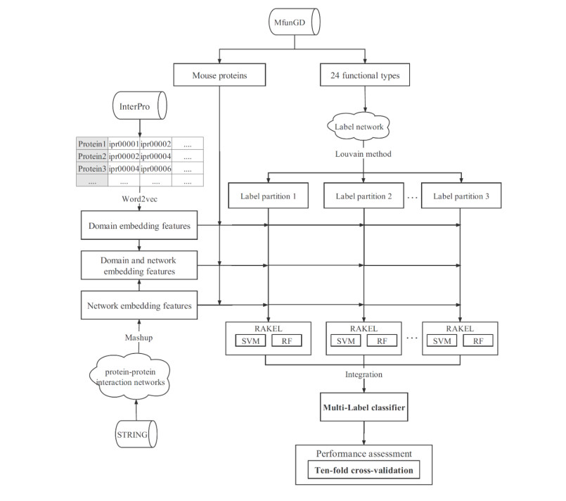
Protein is very important for almost all living creatures because it participates in most complicated and essential biological processes. Determining the functions of given proteins is one of the most essential problems in protein science. Such determination can be conducted through traditional experiments. However, the experimental methods are always time-consuming and of high costs. In recent years, computational methods give useful aids for identification of protein functions. This study presented a new multi-label classifier for identifying functions of mouse proteins. Due to the number of functional types, which were termed as labels in the classification procedure, a label space partition method was employed to divide labels into some partitions. On each partition, a multi-label classifier was constructed. The classifiers based on all partitions were integrated in the proposed classifier. The cross-validation results proved that the proposed classifier was of good performance. Classifiers with label partition were superior to those without label partition or with random label partition.
Citation: Xuan Li, Lin Lu, Lei Chen. Identification of protein functions in mouse with a label space partition method[J]. Mathematical Biosciences and Engineering, 2022, 19(4): 3820-3842. doi: 10.3934/mbe.2022176
Protein is very important for almost all living creatures because it participates in most complicated and essential biological processes. Determining the functions of given proteins is one of the most essential problems in protein science. Such determination can be conducted through traditional experiments. However, the experimental methods are always time-consuming and of high costs. In recent years, computational methods give useful aids for identification of protein functions. This study presented a new multi-label classifier for identifying functions of mouse proteins. Due to the number of functional types, which were termed as labels in the classification procedure, a label space partition method was employed to divide labels into some partitions. On each partition, a multi-label classifier was constructed. The classifiers based on all partitions were integrated in the proposed classifier. The cross-validation results proved that the proposed classifier was of good performance. Classifiers with label partition were superior to those without label partition or with random label partition.

| [1] |
R. Milo, What is the total number of protein molecules per cell volume? A call to rethink some published values, Bioessays, 35 (2013), 1050-1055. https://doi.org/10.1002/bies.201300066 doi: 10.1002/bies.201300066

|
| [2] |
Z. C. Üretmen Kagıalı, A. Şentürk, N. E. Özkan Küçük, M. H. Qureshi, N. Özlü, Proteomics in cell division, Proteomics, 17 (2017), 1600100. https://doi.org/10.1002/pmic.201600100 doi: 10.1002/pmic.201600100
|
| [3] |
M. J. Mughal, R. Mahadevappa, H. F. Kwok, DNA replication licensing proteins: Saints and sinners in cancer, Semin. Cancer Biol., 58 (2019), 11-21. https://doi.org/10.1016/j.semcancer.2018.11.009 doi: 10.1016/j.semcancer.2018.11.009
|
| [4] |
D. Davidi, R. Milo, Lessons on enzyme kinetics from quantitative proteomics, Curr. Opin. Biotechnol., 46 (2017), 81-89. https://doi.org/10.1016/j.copbio.2017.02.007 doi: 10.1016/j.copbio.2017.02.007
|
| [5] |
S. F. Altschul, W. Gish, W. Miller, E. W. Myers, D. J. Lipman, Basic local alignment search tool, J. Mol. Biol., 215 (1990), 403-410. https://doi.org/10.1016/S0022-2836(05)80360-2 doi: 10.1016/S0022-2836(05)80360-2
|
| [6] |
C. J. Sigrist, L. Cerutti, E. De Castro, P. S. Langendijk-Genevaux, V. Bulliard, A. Bairoch, et al., PROSITE, a protein domain database for functional characterization and annotation, Nucleic Acids Res., 38 (2010), D161-D166. https://doi.org/10.1093/nar/gkp885 doi: 10.1093/nar/gkp885
|
| [7] |
R. D. Finn, J. Mistry, B. Schuster-Böckler, S. Griffiths-Jones, V. Hollich, T. Lassmann, et al., Pfam: clans, web tools and services, Nucleic Acids Res., 34 (2006), D247-D251. https://doi.org/10.1093/nar/gkj149 doi: 10.1093/nar/gkj149
|
| [8] |
Y. Ye, A. Godzik, FATCAT: a web server for flexible structure comparison and structure similarity searching, Nucleic Acids Res., 32 (2004), W582-W585. https://doi.org/10.1093/nar/gkh430 doi: 10.1093/nar/gkh430
|
| [9] |
L. Hu, T. Huang, X. Shi, W. C. Lu, Y. D. Cai, K. C. Chou, Predicting functions of proteins in mouse based on weighted protein-protein interaction network and protein hybrid properties, PLoS One, 6 (2011), e14556. https://doi.org/10.1371/journal.pone.0014556 doi: 10.1371/journal.pone.0014556
|
| [10] |
G. Huang, C. Chu, T. Huang, X. Kong, Y. Zhang, N. Zhang, et al., Exploring mouse protein function via multiple approaches, PLoS One, 11 (2016), e0166580. https://doi.org/10.1371/journal.pone.0166580 doi: 10.1371/journal.pone.0166580
|
| [11] |
X. Wang, Y. Wang, Z. Xu, Y. Xiong, D. Q. Wei, ATC-NLSP: Prediction of the classes of anatomical therapeutic chemicals using a network-based label space partition method, Front. Pharmacol., 10 (2019), 971. https://doi.org/10.3389/fphar.2019.00971 doi: 10.3389/fphar.2019.00971
|
| [12] |
X. Wang, X. Zhu, M. Ye, Y. Wang, C. D. Li, Y. Xiong, et al., STS-NLSP: A network-based label space partition method for predicting the specificity of membrane transporter substrates using a hybrid feature of structural and semantic similarity, Front. Bioeng. Biotech., 7 (2019), 306. https://doi.org/10.3389/fbioe.2019.00306 doi: 10.3389/fbioe.2019.00306
|
| [13] |
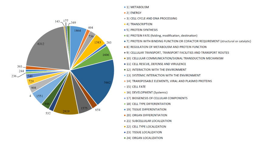
A. Ruepp, O. N. Doudieu, J. van den Oever, B. Brauner, I. Dunger-Kaltenbach, G. Fobo, et al., The mouse functional genome database (MfunGD): functional annotation of proteins in the light of their cellular context, Nucleic Acids Res., 34 (2006), D568-D571. https://doi.org/10.1093/nar/gkj074 doi: 10.1093/nar/gkj074
|
| [14] |
V. D. Blondel, J. L. Guillaume, R. Lambiotte, E. Lefebvre1, Fast unfolding of communities in large networks, J. Stat. Mech-Theory E., 2008 (2008), P10008. https://doi.org/10.1088/1742-5468/2008/10/P10008 doi: 10.1088/1742-5468/2008/10/P10008
|
| [15] | G. Tsoumakas, I. Vlahavas, Random k-Labelsets: An ensemble method for multilabel classification, in European conference on machine learningmachine learning, (2007), 406-417. https://doi.org/10.1007/978-3-540-74958-5_38 |
| [16] |
C. Cortes, V. Vapnik, Support-vector networks, Mach. Learn., 20 (1995), 273-297. https://doi.org/10.1007/BF00994018 doi: 10.1007/BF00994018
|
| [17] |
L, Breiman, Random forests, Mach. Learn., 45 (2001), 5-32. https://doi.org/10.1023/A:1010933404324 doi: 10.1023/A:1010933404324
|
| [18] |
M. Ashburner, S. Lewis, On ontologies for biologists: the Gene Ontology-untangling the web, in Novartis Foundation Symposia (eds. N. Foundation), Wiley Online Library, 247 (2002), 66-80. https://doi.org/10.1002/0470857897.ch6 doi: 10.1002/0470857897.ch6
|
| [19] |
E. Camon, M. Magrane, D. Barrell, D. Binns, W. Fleischmann, P. Kersey, et al., The gene ontology annotation (GOA) project: implementation of GO in SWISS-PROT, TrEMBL, and InterPro, Genome Res., 13 (2003), 662-672. https://doi.org/10.1101/gr.461403 doi: 10.1101/gr.461403
|
| [20] |
K. C. Chou, Y. D. Cai, Using functional domain composition and support vector machines for prediction of protein subcellular location, J. Biol. Chem., 277 (2002), 45765-45769. https://doi.org/10.1074/jbc.M204161200 doi: 10.1074/jbc.M204161200
|
| [21] |
K. C. Chou, Y. D. Cai, Predicting protein structural class by functional domain composition, Biochem, Bioph. Res. Co., 321 (2004), 1007-1009. https://doi.org/10.1016/j.bbrc.2004.07.059 doi: 10.1016/j.bbrc.2004.07.059
|
| [22] |
L. Lu, Z. Qian, Y. D. Cai, Y. Li, ECS: an automatic enzyme classifier based on functional domain composition, Comput. Biol. Chem., 31 (2007), 226-232. https://doi.org/10.1016/j.compbiolchem.2007.03.008 doi: 10.1016/j.compbiolchem.2007.03.008
|
| [23] |
H. Zhou, Y. Yang, H. B. Shen, Hum-mPLoc 3.0: prediction enhancement of human protein subcellular localization through modeling the hidden correlations of gene ontology and functional domain features, Bioinformatics, 33 (2017), 843-853. https://doi.org/10.1093/bioinformatics/btw723 doi: 10.1093/bioinformatics/btw723
|
| [24] | L. Chen, K. Y. Feng, Y. D. Cai, K. C. Chou, H. P. Li, Predicting the network of substrate-enzyme-product triads by combining compound similarity and functional domain composition, BMC Bioinformatics, 11 (2010), 293. https://doi.org/10.1186/1471-2105-11-293 |
| [25] |
M. Blum, H. Y. Chang, S. Chuguransky, T. Grego, S. Kandasaamy, A. Mitchell, et al., The InterPro protein families and domains database: 20 years on, Nucleic Acids Res., 49 (2021), D344-D354. https://doi.org/10.1093/nar/gkaa977 doi: 10.1093/nar/gkaa977
|
| [26] | T. Mikolov, K. Chen, G. Corrado, J. Dean, Efficient estimation of word representations in vector space, Preprint, arXiv: 1301.3781v3. |
| [27] |
K. W. Church, Word2Vec, Nat. Lang. Eng., 23 (2017), 155-162. https://doi.org/10.1017/S1351324916000334 doi: 10.1017/S1351324916000334
|
| [28] | B. Perozzi, R. Al-Rfou, S. Skiena, Deepwalk: Online learning of social representations, in 20th ACM SIGKDD International Conference on Knowledge Discovery and Data Mining, (2014), 701-710. https://doi.org/10.1145/2623330.2623732 |
| [29] | A. Grover, J. Leskovec, node2vec: Scalable feature learning for networks, in 22nd ACM SIGKDD International Conference on Knowledge Discovery and Data Mining, (2016), 855-864. https://doi.org/10.1145/2939672.2939754 |
| [30] |
H. Cho, B. Berger, J. Peng, Compact integration of multi-network topology for functional analysis of genes, Cell Syst., 3 (2016), 540-548. https://doi.org/10.1016/j.cels.2016.10.017 doi: 10.1016/j.cels.2016.10.017
|
| [31] |
H. Liu, B. Hu, L. Chen, L. Lu, Identifying protein subcellular location with embedding features learned from networks, Curr. Proteomics, 18 (2021): 646-660. https://doi.org/10.2174/1570164617999201124142950 doi: 10.2174/1570164617999201124142950
|
| [32] |
X. Zhang, L. Chen, Z. H. Guo, H. Liang, Identification of human membrane protein types by incorporating network embedding methods, IEEE Access, 7 (2019), 140794-140805. https://doi.org/10.1109/ACCESS.2019.2944177 doi: 10.1109/ACCESS.2019.2944177
|
| [33] | X. Pan, L. Chen, M. Liu, Z. Niu, T. Huang, Y. D. Cai, Identifying protein subcellular locations with embeddings-based node2loc, IEEE ACM Trans. Comput. Bi., 2021 (2021). https://doi.org/10.1109/TCBB.2021.3080386 |
| [34] |
X. Pan, H. Li, T. Zeng, Z. Li, L. Chen, T. Huang, et al., Identification of protein subcellular localization with network and functional embeddings, Front. Genet., 11 (2021), 626500. https://doi.org/10.3389/fgene.2020.626500 doi: 10.3389/fgene.2020.626500
|
| [35] |
D. Szklarczyk, A. Franceschini, S. Wyder, K. Forslund, D. Heller, J. Huerta-Cepas, et al., STRING v10: protein–protein interaction networks, integrated over the tree of life, Nucleic Acids Res., 43 (2015), D447-D452. https://doi.org/10.1093/nar/gku1003 doi: 10.1093/nar/gku1003
|
| [36] | H. Tong, C. Faloutsos, J. Pan, Fast random walk with restart and its applications, in Sixth International Conference on Data Mining, (2006), 613-622. https://doi.org/10.1109/ICDM.2006.70 |
| [37] |
S. Kohler, S. Bauer, D. Horn, P. N. Robinson, Walking the interactome for prioritization of candidate disease genes, Am. J. Hum. Genet., 82 (2008), 949-958. https://doi.org/10.1016/j.ajhg.2008.02.013 doi: 10.1016/j.ajhg.2008.02.013
|
| [38] | G. Tsoumakas, I. Katakis, Multi-label classification: An overview. Int. J. Data Warehous., 3 (2007), 1-13. |
| [39] | J. Read, P. Reutemann, B. Pfahringer, G. Holmes, MEKA: A multi-label/multi-target extension to WEKA, J. Mach. Learn. Res., 17 (2016), 1-5. |
| [40] |
J. P. Zhou, L. Chen, Z. H. Guo, iATC-NRAKEL: An efficient multi-label classifier for recognizing anatomical therapeutic chemical classes of drugs, Bioinformatics, 36 (2020), 1391-1396. https://doi.org/10.1093/bioinformatics/btz757 doi: 10.1093/bioinformatics/btz757
|
| [41] |
L. Chen, S. Wang, Y. H. Zhang, L. Li, Z. H. Xing, J. Yang, et al., Identify key sequence features to improve CRISPR sgRNA efficacy, IEEE Access, 5 (2017), 26582-26590. https://doi.org/10.1109/ACCESS.2017.2775703 doi: 10.1109/ACCESS.2017.2775703
|
| [42] |
J. P. Zhou, L. Chen, T. Wang, M. Liu, iATC-FRAKEL: A simple multi-label web-server for recognizing anatomical therapeutic chemical classes of drugs with their fingerprints only, Bioinformatics, 36 (2020), 3568-3569. https://doi.org/10.1093/bioinformatics/btaa166 doi: 10.1093/bioinformatics/btaa166
|
| [43] |
Y. H. Zhang, H. Li, T. Zeng, L. Chen, Z. Li, T. Huang, et al., Identifying transcriptomic signatures and rules for SARS-CoV-2 infection, Front. Cell Dev. Biol., 8 (2021), 627302. https://doi.org/10.3389/fcell.2020.627302 doi: 10.3389/fcell.2020.627302
|
| [44] |
Y. H. Zhang, Z. Li, T. Zeng, L. Chen, H. Li, T. Huang, et al., Detecting the multiomics signatures of factor-specific inflammatory effects on airway smooth muscles, Front. Genet., 11 (2021), 599970. https://doi.org/10.3389/fgene.2020.599970 doi: 10.3389/fgene.2020.599970
|
| [45] |
Y. Zhu, B. Hu, L. Chen, Q. Dai, iMPTCE-Hnetwork: a multi-label classifier for identifying metabolic pathway types of chemicals and enzymes with a heterogeneous network, Comput. Math. Method M., 2021 (2021), 6683051. https://doi.org/10.1155/2021/6683051 doi: 10.1155/2021/6683051
|
| [46] |
Y. Wang, Y. Xu, Z. Yang, X. Liu, Q. Dai, Using recursive feature selection with random forest to improve protein structural class prediction for low-similarity sequences, Comput. Math. Method M., 2021 (2021), 5529389. https://doi.org/10.1155/2021/5529389 doi: 10.1155/2021/5529389
|
| [47] | J. Platt, Fast training of support vector machines using sequential minimal optimization, MIT Press, 1998. |
| [48] |
Y. Yang, L. Chen, Identification of drug-disease associations by using multiple drug and disease networks, Curr. Bioinform., 17 (2022), 48-59. https://doi.org/10.2174/1574893616666210825115406 doi: 10.2174/1574893616666210825115406
|
| [49] |
Y. Jia, R. Zhao, L. Chen, Similarity-based machine learning model for predicting the metabolic pathways of compounds, IEEE Access, 8 (2020), 130687-130696. https://doi.org/10.1109/ACCESS.2020.3009439 doi: 10.1109/ACCESS.2020.3009439
|
| [50] |
X. Zhao, L. Chen, J. Lu, A similarity-based method for prediction of drug side effects with heterogeneous information, Math. Biosci., 306 (2018), 136-144. https://doi.org/10.1016/j.mbs.2018.09.010 doi: 10.1016/j.mbs.2018.09.010
|
| [51] |
K. K. Kandaswamy, K. C. Chou, T. Martinetz, S. Möllera, P. N. Suganthand, S. Sridharan, et al., AFP-Pred: A random forest approach for predicting antifreeze proteins from sequence-derived properties, J. Theor. Biol., 270 (2011), 56-62. https://doi.org/10.1016/j.jtbi.2010.10.037 doi: 10.1016/j.jtbi.2010.10.037
|
| [52] |
Y. B. Marques, A. de Paiva Oliveira, A. T. Ribeiro Vasconcelos, F. R. Cerqueira, Mirnacle: machine learning with SMOTE and random forest for improving selectivity in pre-miRNA ab initio prediction, BMC Bioinformatics, 17 (2016), 474. http://dx.doi.org/10.1186/s12859-017-1508-0 doi: 10.1186/s12859-017-1508-0
|
| [53] |
G. Pugalenthi, K. Kandaswamy, K. C. Chou, S. Vivekanandan, P. Kolatkar, RSARF: Prediction of residue solvent accessibility from protein sequence using random forest method, Protein Peptide Lett., 19 (2011), 50-56. https://doi.org/10.2174/092986612798472875 doi: 10.2174/092986612798472875
|
| [54] |
M. Onesime, Z. Yang, Q. Dai, Genomic island prediction via chi-square test and random forest algorithm, Comput. Math. Method M., 2021 (2021), 9969751. https://doi.org/10.1155/2021/9969751 doi: 10.1155/2021/9969751
|
| [55] | M. Fernandez-Delgado, E. Cernadas, S. Barro, D. Amorim, Do we need hundreds of classifiers to solve real world classification problems?, J. Mach. Learn. Res., 15 (2014), 3133-3181. |
| [56] | R. Kohavi, A study of cross-validation and bootstrap for accuracy estimation and model selection, in International Joint Conference on Artificial Intelligence, (1995), 1137-1145. |
| [57] |
W. Chen, L. Chen, Q. Dai, iMPT-FDNPL: identification of membrane protein types with functional domains and a natural language processing approach, Comput. Math. Method M., 2021 (2021), 7681497. https://doi.org/10.1155/2021/7681497 doi: 10.1155/2021/7681497
|
| [58] |
J. Zhang, Q. Chen, B. Liu, iDRBP_MMC: Identifying DNA-binding proteins and RNA-binding proteins based on multi-label learning model and motif-based convolutional neural network, J. Mol. Biol., 432 (2020), 5860-5875. https://doi.org/10.1016/j.jmb.2020.09.008 doi: 10.1016/j.jmb.2020.09.008
|
Figures(9) / Tables(6)

Xuan Li, Lin Lu, Lei Chen. Identification of protein functions in mouse with a label space partition method[J]. Mathematical Biosciences and Engineering, 2022, 19(4): 3820-3842. doi: 10.3934/mbe.2022176


 DownLoad: