A novel design of Gudermannian function as a neural network for the singular nonlinear delayed, prediction and pantograph differential models

Zulqurnain Sabir; Hafiz Abdul Wahab; Juan L.G. Guirao; Zulqurnain Sabir; Hafiz Abdul Wahab; Juan L.G. Guirao

doi:10.3934/mbe.2022030

Mathematical Biosciences and Engineering

2022, Volume 19, Issue 1: 663-687. doi: 10.3934/mbe.2022030

Previous Article Next Article

Research article Special Issues

A novel design of Gudermannian function as a neural network for the singular nonlinear delayed, prediction and pantograph differential models

1.
Department of Mathematics and Statistics, Hazara University, Mansehra, Pakistan
2.
Department of Applied Mathematics and Statistics, Technical University of Cartagena, Hospital de Marina 30203-Cartagena, Spain
3.
Nonlinear Analysis and Applied Mathematics (NAAM)-Research Group, Department of Mathematics, Faculty of Science, King Abdulaziz University, P. O. Box 80203, Jeddah 21589, Saudi Arabia

Academic Editor: Haiyan Wang

Received: 30 July 2021 Accepted: 28 October 2021 Published: 19 November 2021

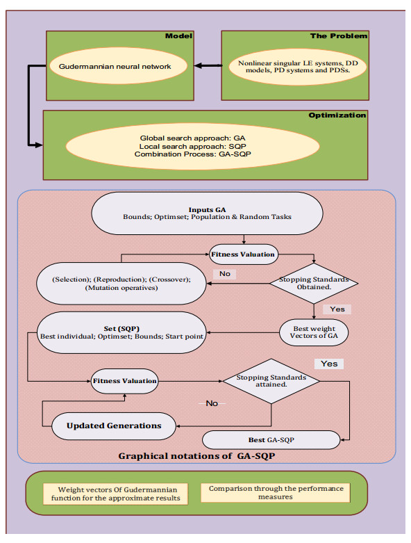
The present work is to solve the nonlinear singular models using the framework of the stochastic computing approaches. The purpose of these investigations is not only focused to solve the singular models, but the solution of these models will be presented to the extended form of the delayed, prediction and pantograph differential models. The Gudermannian function is designed using the neural networks optimized through the global scheme "genetic algorithms (GA)", local method "sequential quadratic programming (SQP)" and the hybridization of GA-SQP. The comparison of the singular equations will be presented with the exact solutions along with the extended form of delayed, prediction and pantograph based on these singular models. Moreover, the neuron analysis will be provided to authenticate the efficiency and complexity of the designed approach. For the correctness and effectiveness of the proposed approach, the plots of absolute error will be drawn for the singular delayed, prediction and pantograph differential models. For the reliability and stability of the proposed method, the statistical performances "Theil inequality coefficient", "variance account for" and "mean absolute deviation'' are observed for multiple executions to solve singular delayed, prediction and pantograph differential models.

Keywords:

Citation: Zulqurnain Sabir, Hafiz Abdul Wahab, Juan L.G. Guirao. A novel design of Gudermannian function as a neural network for the singular nonlinear delayed, prediction and pantograph differential models[J]. Mathematical Biosciences and Engineering, 2022, 19(1): 663-687. doi: 10.3934/mbe.2022030

Related Papers:

[1]	Zulqurnain Sabir, Muhammad Asif Zahoor Raja, Abeer S. Alnahdi, Mdi Begum Jeelani, M. A. Abdelkawy . Numerical investigations of the nonlinear smoke model using the Gudermannian neural networks. Mathematical Biosciences and Engineering, 2022, 19(1): 351-370. doi: 10.3934/mbe.2022018
[2]	Reymundo Itzá Balam, Francisco Hernandez-Lopez, Joel Trejo-Sánchez, Miguel Uh Zapata . An immersed boundary neural network for solving elliptic equations with singular forces on arbitrary domains. Mathematical Biosciences and Engineering, 2021, 18(1): 22-56. doi: 10.3934/mbe.2021002
[3]	Zulqurnain Sabir, Muhammad Asif Zahoor Raja, Aldawoud Kamal, Juan L.G. Guirao, Dac-Nhuong Le, Tareq Saeed, Mohamad Salama . Neuro-Swarm heuristic using interior-point algorithm to solve a third kind of multi-singular nonlinear system. Mathematical Biosciences and Engineering, 2021, 18(5): 5285-5308. doi: 10.3934/mbe.2021268
[4]	Thomas Torku, Abdul Khaliq, Fathalla Rihan . SEINN: A deep learning algorithm for the stochastic epidemic model. Mathematical Biosciences and Engineering, 2023, 20(9): 16330-16361. doi: 10.3934/mbe.2023729
[5]	Diego Fasoli, Stefano Panzeri . Mathematical studies of the dynamics of finite-size binary neural networks: A review of recent progress. Mathematical Biosciences and Engineering, 2019, 16(6): 8025-8059. doi: 10.3934/mbe.2019404
[6]	Pan Wang, Xuechen Li, Qianqian Zheng . Synchronization of inertial complex-valued memristor-based neural networks with time-varying delays. Mathematical Biosciences and Engineering, 2024, 21(2): 3319-3334. doi: 10.3934/mbe.2024147
[7]	Hongqiang Zhu . A graph neural network-enhanced knowledge graph framework for intelligent analysis of policing cases. Mathematical Biosciences and Engineering, 2023, 20(7): 11585-11604. doi: 10.3934/mbe.2023514
[8]	Hang Yu, Jiarui Shi, Jin Qian, Shi Wang, Sheng Li . Single dendritic neural classification with an effective spherical search-based whale learning algorithm. Mathematical Biosciences and Engineering, 2023, 20(4): 7594-7632. doi: 10.3934/mbe.2023328
[9]	Jing Cao, Dong Zhao, Chenlei Tian, Ting Jin, Fei Song . Adopting improved Adam optimizer to train dendritic neuron model for water quality prediction. Mathematical Biosciences and Engineering, 2023, 20(5): 9489-9510. doi: 10.3934/mbe.2023417
[10]	Ravi Agarwal, Snezhana Hristova, Donal O’Regan, Radoslava Terzieva . Stability properties of neural networks with non-instantaneous impulses. Mathematical Biosciences and Engineering, 2019, 16(3): 1210-1227. doi: 10.3934/mbe.2019058

Abstract

1. Introduction

The models based on Lane-Emden (LE) have a variety of valuable applications in physiological, physical models, mathematics science and engineering studies. The celebrated form of the LE has a great significance due to the singular point and this model is explored by famous scientists Lane and Emden ^[1,2] working on the thermal gas performance and the thermodynamics state ^[3]. The literature/generic form of the LE model is given as ^[4,5,6,7]:

$\left\{ \begin{array}{l} \frac{{{d^2}\aleph }}{{d{\tau ^2}}} + \frac{\upsilon }{\tau }\frac{{d\aleph }}{{d\tau }} + g(\tau , \aleph ) = f(\tau ), \, \, \, \, \, \upsilon \geqslant 0, \, \, 0 < \tau \leqslant 1, \hfill \\ \aleph (0) = {u_1}, \, \, \frac{{d\aleph (0)}}{{d\tau }} = {u_2}, \, \, \hfill \end{array} \right.$

(1)

where $\upsilon$ is the shape factor, $g(\tau, \aleph)$ is the continuous real valued based function, ${u_1}$ and ${u_2}$ are the initial conditions (ICs).

The LE based singular nonlinear systems define an area of physical sciences ^[8], gaseous density stars ^[9], stellar models ^[10], morphogenesis ^[11], oscillating fields ^[12], mathematical systems ^[13], dusty fluidics ^[14] and an isotropic source ^[15]. To present the solutions of the singular systems is not easy and considered tough due to the involvement of singularity at the origin. Only a few schemes in literature are available to solve the singular based LE types of models ^[16,17].

A variety of physical phenomena are investigated using the sense of differential systems, among them the delay differential (DD) form is the most prominent due to the vast applications in technology as well as engineering. The DD systems were introduced few centuries ago and has number of applications in the variety of scientific areas including a communication system, engineering models, population dynamics, transport systems and economic circumstances ^{[18,19,20,21]}. Few associated investigations of DD systems are the geometric functions reliability through DD systems to exploit the factors of delay-dependent studied by Beretta et al. ^[22]. The biological based mathematical systems based on the DD models were studied by the Forde ^[23]. The implementations based on the Galerkin wavelet scheme together with the Taylor series investigations to obtain the numerical outcomes of the DD system defined by the Frazier ^[24]. The coupled variation iteration approach to calculate the analytical outcomes of the DD system introduced by Rangkuti et al. ^[25]. The Runge-Kutta approach to calculate the numerical procedures of the DD systems is implemented by the Chapra ^[26]. Few more schemes have been implemented to solve the DD models are reported in the literature ^[27,28,29]. The PD system is considered using the ideas of the DD system. The prediction differential system is applied in weather forecasting, transport, stock markets, technology, engineering, astrophysics and biological networks ^[30]. The literature form of the DD and PD systems are provided in Eqs (2) and (3) as ^[31]:

$\left\{ \begin{array}{l} \frac{{{d^2}\aleph }}{{d{\tau ^2}}} = h\left( {\tau , \, \aleph (\tau ), \, \aleph (\tau - {r_1})} \right), \;\;\;\; {r_1} > 0, \, \, l \leqslant \tau \leqslant m, \hfill \\ \aleph (\tau ) = \phi (\tau ), \;\;\;\; \varepsilon \leqslant \tau \leqslant l, \;\;\;\;\;\;\; 0 \leqslant {r_1} \leqslant \left| {l - \varepsilon } \right|, \hfill \\ \frac{{d\aleph (l)}}{{d\tau }} = w, \hfill \end{array} \right.$

(2)

where $\phi (\tau)$ shows the ICs and $\aleph (\tau - {r_1})$ represents the delayed form, while ${r_1}$ is delayed term, l and m are constants. The term w is the value derivative of $\aleph$ at l and $\varepsilon$ represents a small positive constant. As $\varepsilon \leqslant \tau \leqslant l$ , then the necessary condition for the delay term bound should be 0 ≤ r1 ≤ | l − ε | such that system in Eq (2), remained DD equation.

When any of the value is added in $\tau$ , it becomes prediction, i.e., $\aleph (\tau + {r_1})$ , where $r$ is used as a prediction term and PD system is given as:

$\left\{ \begin{array}{l} \frac{{{d^2}\aleph }}{{d{\tau ^2}}} = h\left( {\tau , \, \aleph (\tau ), \, \aleph (\tau + {r_1})} \right), \;\;\;\;\; {r_1} > 0, \, \, l \leqslant \tau \leqslant m, \hfill \\ \aleph (\tau ) = \phi (\tau ), \;\;\;\;\;\varepsilon \leqslant \tau \leqslant l,\;\;\;\;\;\;\;\;0 \leqslant {r_1} \leqslant \left| {\varepsilon - l} \right|, \hfill \\ \frac{{d\aleph (l)}}{{d\tau }} = w, \hfill \end{array} \right.$

(3)

The pantograph differential systems (PDSs) have a variety of submission due to its enormous significance in the engineering fields, biological models and science areas. Some well-known applications are light absorption in the solid, dynamical population networks, communication networks, control systems, infectious viruses, propagation systems, electronic frameworks, transports and quantum mechanism ^{[32,33,34,35,36]}. There are various techniques that have been implemented to treat the PDSs, e.g., one-dimensional transformation approach, Taylor polynomial method and Direchlet series scheme ^{[37,38,39,40,41]}. The generic form of the PDSs is given as:

$\left\{ \begin{array}{l} \beta \frac{{{d^2}}}{{d{\tau ^2}}}\aleph (\beta \tau ) + \frac{\upsilon }{\tau }\frac{d}{{d\tau }}\aleph (\beta \tau ) + g(\tau , \aleph ) = f(\tau ), & \, \upsilon \geqslant 0, \, \, 0 < \tau \leqslant 1, \hfill \\ \aleph (0) = {u_1}, \, \, \frac{{d\aleph (0)}}{{d\tau }} = {u_2}, \hfill \end{array} \right.$

(4)

For solving the LE based singular systems, every technique has specific sensitivity, correctness, potential and efficiency, over and above, flaws, demerits and weaknesses. The wide-ranging computing potential schemes are used for the singular LE systems, DD models, PD systems and PDSs. To solve these singular systems, Gudermannian function is designed as a neural network optimized with the global scheme "genetic algorithms (GA)", local method "sequential quadratic programming (SQP)" and the hybridization of GA-SQP. The stochastic numerical schemes have been explored to solve various applications like HIV infection nonlinear system based infected latently cells ^{[42,43,44,45]}, higher order singular nonlinear systems ^[46,47,48], mosquito dispersal nonlinear system ^[49], heat conduction system based human head ^[50], doubly singular systems ^[51,52] and SIR nonlinear dengue fever system ^[53].These well-known submissions authenticated the implication of the stochastic computing solvers in terms of stability, exactitude and convergence. Hence, the design of Gudermannian function that work as a neural network is never been applied to solve the LE systems, DD models, PD systems and PDSs by using the optimization through the GA-SQP procedures. Some novel topographies of the proposed Gudermannian neural network along with GA-SQP are summarized as:

● A novel Gudermannian function is designed as a neural network is presented for solving the singular LE systems, DD models, PD systems and PDSs by using the optimization through the GA-SQP procedures.

● The numerical solutions of the stochastic procedures for solving four different examples of the singular systems are found precise and accurate.

● The analysis based on small and large neurons are effectively provided to authenticate the efficiency and complexity of the designed approach.

● The matching of the best and mean outcomes obtained by the stochastic procedures authenticate the consistency, accuracy and perfection of the singular LE systems, DD models, PD systems and PDSs.

● The reliability of the outcomes obtained by the proposed stochastic procedures through single/multiple executions via performance operators based on mean, Theil inequality coefficient (TIC), median (Med), variance account for (VAF), semi-interquartile range (SIR), maximum (Max) and mean absolute deviation (MAD) improve the capability of the scheme.

The remaining parts of the paper are given as: Section 2 labels the designed structure along with the statistical performance, Section 3 indicates the details of numerical results together with clarifications of the results. The neuron analysis will be presented in Section 4. The concluding remarks are provided in the last Section.

2. Methodology

In this section, the Gudermannian function is presented as a neural network for the singular LE systems, DD models, PD systems and PDSs by using the optimization through the GA-SQP procedures. The differential operators, objective function and optimization-based procedures using the proposed scheme are also presented.

2.1. Designed procedures through Gudermannian function as a neural network

The artificial neural networks are considered important to form the consistent and steadfast solutions for frequent submission arising in the various fields. In this modelling, $\hat \aleph (\tau)$ indicates the obtained performances via the Gudermannian function as a neural network and its derivatives are described as:

$\hat \aleph (\tau ) = \sum\limits_{m\, = \, 1}^k {{s_m}y({w_m}\tau + {z_m})}$

${\hat \aleph ^{(n)}}(\tau ) = \sum\limits_{m\, = \, 1}^k {{s_m}{y^{(n)}}({w_m}\tau + {z_m})}$

(5)

where, k shows the neurons and n represents the derivative. The objective function is y, whereas, s, $w$ , $z$ are the unidentified weights that are $\mathit{\boldsymbol{W}} = [\mathit{\boldsymbol{s}}, \mathit{\boldsymbol{w}}, \mathit{\boldsymbol{z}}]$ , for $\mathit{\boldsymbol{s}} = [{s_1}, {s_2}, {s_3}, ..., {s_k}]$ , $\mathit{\boldsymbol{w}} = [{w_1}, {w_2}, {w_3}, ..., {w_k}]$ and $\mathit{\boldsymbol{z}} = [{z_1}, {z_2}, {z_3}, ..., {z_k}]$ . The mathematical form of the Gudermannian function is given as:

$y(\tau ) = 2{\tan ^{ - 1}}{e^\tau } - 0.5\pi$

(6)

The approximate form of the continuous mapping based differential operations is shown as:

$\hat \aleph (\tau ) = \sum\limits_{m = 1}^k {{s_m}\left( {2{{\tan }^{ - 1}}{e^{({w_m}\tau + {z_m})}} - 0.5\pi } \right)} ,$

$\hat \aleph '(\tau ) = \sum\limits_{m = 1}^k {2{s_m}{w_m}\left( {\frac{{{e^{({w_m}\tau + {z_m})}}}}{{1 + {{\left( {{e^{({w_m}\tau + {z_m})}}} \right)}^2}}}} \right)} ,$

(7)

$\hat \aleph ''(\tau ) = \sum\limits_{m = 1}^k {2{s_m}w_m^2\left( {\frac{{{e^{({w_m}\tau + {z_m})}}}}{{1 + {{\left( {{e^{({w_m}\tau + {z_m})}}} \right)}^2}}} - \frac{{2{e^{{{({w_m}\tau + {z_m})}^3}}}}}{{{{\left( {1 + {{\left( {{e^{({w_m}\tau + {z_m})}}} \right)}^2}} \right)}^2}}}} \right)} ,$

To solve the singular LE systems, DD models, PD systems and PDSs, the objective function is formulated in terms of mean squared error, which is written as:

${E_{Fit}} = {E_{Fit - 1}} + {E_{Fit - 2}},$

(8)

where ${E_{Fit}}$ is an unsupervised learning-based error function related to the LE systems, DD models, PD systems and PDSs. ${E_{Fit - 1}}$ and ${E_{Fit - 2}}$ are the error based objective functions based on the differential model and ICs of the system (1)–(4). The fitness function ${E_{Fit - 1}}$ is constructed using the system (1), while for the system (2)–(4) can also be constructed.

${E_{Fit - 1}} = \frac{1}{N}{\sum\limits_{i = 1}^N {\left( {\frac{{{d^2}\hat \aleph ({\tau _i})}}{{d{\tau ^2}}} + \frac{\upsilon }{{{\tau _i}}}\frac{{d\hat \aleph ({\tau _i})}}{{d\tau }} + g\left( {{\tau _i}, \hat \aleph ({\tau _i})} \right) - f({\tau _i})\, } \right)} ^2},$

(9)

${E_{Fit - 2}} = \frac{1}{2}\left( {{{({{\hat \aleph }_0} - {u_1})}^2} + \, {{\left( {\frac{{d{{\hat \aleph }_0}}}{{d\tau }} - {u_2}} \right)}^2}\, } \right),$

(10)

where $Nh = 1, \, \, g(\tau, \aleph) = g({\tau _i}, \aleph ({\tau _i}))$ and ${\tau _i}\, = ih$ .

2.2. Network optimization GA-SQP

In this section, the Gudermannian function as a neural network is designed and numerical solutions for solving the singular LE systems, DD models, PD systems and PDSs through the optimization of GA-SQP are presented.

The evolutionary intelligent computing approach "GA" is designed on the basis of natural growth. GA is introduced by Holland in the previous century and then it is used as a leading factor in optimization using the constrained/unconstrained systems ^[54]. GA shows the optimal performances of mutation, crossover, heuristic and selection and broadly implemented in various fields of robotics, Bioinformatics, optics, astrophysics, digital communication, financial based mathematics, signal processing, nuclear based power systems, chemical industry and economics. Recently, it is implemented in the optimization of wind power systems ^[55], pipe networks ^[56], intrusion detection system ^[57], energy management models ^[58], circularity error unified evaluation ^[59], heterogeneous celebration ^[60], drying process of carrot ^[61], 2D industrial packing problems ^[62] and aquatic weed systems ^[63]. These reputed submissions inspired the authors to optimize through GA the singular LE systems, DD models, PD systems and PDSs for finding the best proposed outputs.

The hybridization of global search with any local search method performs the rapid convergence using the hybridize with the local search scheme. The best GA values are assigned as an initial input. The local search SQP is applied to normalize the parameters. SQP has been applied in various directions, e.g., bilinear model predictive control of a HVAC system ^[64], optimization of the engineering models ^[65], optimal control of building HVAC & R systems ^[66], ESP-implemented wells ^[67], optimal coordination of automated vehicles at intersections ^[68], dynamic combined economic emission dispatch models ^[69], cost minimization of a hybrid photovoltaic, diesel generator, and battery energy storage system ^[70].

Figure 1 indicates the graphical illustrations based Gudermannian function as a neural network and optimization procedures of GA-SQP, while the details of the optimization steps based on GA-SQP are given in Table 1 for singular LE systems, DD models, PD systems and PDSs. The settings of the parameter are adopted based on the experiments, experience, performance advantages and knowledge using different applications in the current work.

Figure 1. Graphical illustrations of the Gudermannian function as a neural network for the singular LE systems, DD models, PD systems and PDSs using the optimization-based GA-SQP.

DownLoad: Full-Size Img PowerPoint

Table 1. Optimization procedures of the designed scheme for the nonlinear singular LE systems, DD models, PD systems and PDSs.

[GA procedures]

Inputs: The chromosomes are defined with equal network entries as:

$\mathit{\boldsymbol{W}} = [\mathit{\boldsymbol{s}}, \mathit{\boldsymbol{w}}, \mathit{\boldsymbol{z}}]$
Population: The chromosomes vectors are indicated as:

$\mathit{\boldsymbol{s}} = [{s_1}, {s_2}, {s_3}, ..., {s_k}]$ ,

$\mathit{\boldsymbol{w}} = [{w_1}, {w_2}, {w_3}, ..., {w_k}]$ and

$\mathit{\boldsymbol{z}} = [{z_1}, {z_2}, {z_3}, ..., {z_k}]$ .
   Output: The global best weight vectors are W_GA-Best
   Initialization: Form a W, which is a weight vector having real elements to choose a chromosome. For the initial population, the design of 'W' is presented. To regulate the generations and assertions for the gaoptimset.
   Fitness assessment: Proficient the fitness (E_Fit) in population for W using Eqs (8)–(10).
   Stopping standards: Terminate if any forms is obtained
       • [E_Fit = 10^–20], [StallLimit = 150], [TolFun = TolCon = 10^–18], [PopulationSize = 285], [Generations = 90].
       • Other values: default
  Go to [storage], if stopping criteria meets
   Ranking: Rank the W to achieve E_Fit
   Reproduction:
       • [Selection~@uniform], [Mutations~adaptfeasible] & [Crossover~heuristic].
   Store: Save W_GA-Best, E_Fit, Generations, time and function counts.
End of [GA] process

Process of SQP
   Inputs: Input: W_GA-Best
  Output: Best GA-SQP are indicated as W_GA-SQP.
   Initialize: Use W_GA-Best, Bounded constraints, assignments, generations and other decelerations.
   Terminate: The procedure stops, if any on the below procedure obtains [E_Fit = 10^–17], [Iterations = 650], [TolCon = TolX = TolFun = 10^–22], [MaxEvalsFun = 286000], While [Stop]
  Fitness assessment: Evaluate the E_Fit, W, using Eqs (8)–(10). Modifications: Using the SQP, Invoke [fmincon]
   Accumulate
  Adjust count of function, W_GA-Best, time, iterations and E_Fit for the present values of SQP.
End of SQP
Data Generations
  The process of GASQP is replicate 50 times for a larger dataset for the singular LE systems, DD models, PD systems and PDSs using the optimization-based GA-SQP through the statistical clarifications.

| Show Table

DownLoad: CSV

2.3. Performance procedures

In this section, the performances through different statistical gages T.I.C, VAF, S.I.R and MAD is provided to validate the constancy and reliability of the proposed Gudermannian function as a neural network using the optimizations of GA-SQP for solving the nonlinear singular LE systems, DD models, PD systems and PDSs. The mathematical formulations of these measures are provided as:

${\text{T}}{\text{.I}}{\text{.C = }}\frac{{\sqrt {\frac{1}{n}{{\sum\limits_{i = 1}^k {\left( {{\aleph _i} - {{\hat \aleph }_i}} \right)} }^2}} }}{{\left( {\sqrt {\frac{1}{n}\sum\limits_{i = 1}^k {\aleph _i^2} } + \sqrt {\frac{1}{n}\sum\limits_{i = 1}^k {\hat \aleph _i^2} } } \right)}},$

(11)

$\left\{ \begin{array}{l} VAF = \left( {1 - \frac{{{var} \left( {{\aleph _i} - {{\hat \aleph }_i}} \right)}}{{{var} \left( {{\aleph _i}} \right)}}} \right) \times 100, \hfill \\ EVAF = \left| {VAF - 100} \right|, \hfill \end{array} \right.$

(12)

$\left\{ \begin{array}{l} {\text{S}}{\text{.I}}{\text{.R}} = - 0.5 \times \left( {{Q_1} - {Q_3}} \right), \hfill \\ {Q_1}{\text{ = }}{1^{st}}\, {\text{quartile}}\, \, {\rm{\& }}\, \, \, {Q_3}\, = {3^{rd}}{\text{ quartile, }}\, \hfill \end{array} \right.$

(13)

${\text{MAD = }}\sum\limits_{i = 1}^k {\left| {{\aleph _i} - {{\hat \aleph }_i}} \right|}$

(14)

3. Simulations of the results and discussions

In this section, the simulation of the results and comprehensive discussions is performed to solve the singular LE systems, DD models, PD systems and PDSs by exploiting the Gudermannian function as a neural network along with the optimal performances of GA-SQP. One example of each nonlinear singular model based on the singular LE systems, DD models, PD systems and PDSs along with the statistical procedures is numerically discussed through the designed scheme.

Problem Ⅰ: Consider a nonlinear singular differential model having an exponential function

$\left\{ \begin{array}{l} \frac{{{d^2}\aleph }}{{d{\tau ^2}}} + \frac{{0.5}}{\tau }\frac{{d\aleph }}{{d\tau }} + ({e^{2\aleph (\tau )}} - 0.5{e^{\aleph (\tau )}}) = 0, \, \, \, \hfill \\ \aleph (0) = \log (2), \, \, \, \aleph (1) = 0.\, \, \hfill \end{array} \right.$

(15)

The fitness function of the above function is given as:

${E_{Fit}} = \frac{1}{N}{\sum\limits_{i = 1}^N {\left( {{\tau _i}\frac{{{d^2}\hat \aleph ({\tau _i})}}{{d{\tau ^2}}} + 0.5\frac{{d\hat \aleph ({\tau _i})}}{{d\tau }} + {\tau _i}({e^{2\hat \aleph ({\tau _i})}} - 0.5{e^{\hat \aleph ({\tau _i})}})} \right)} ^2} + \frac{1}{2}\left( {{{\left( {{{\hat \aleph }_0} - \log (2)} \right)}^2} + {{\left( {{{\hat \aleph }_N}} \right)}^2}} \right).$

(16)

The exact form of the solution is $\log 2 - \log ({\tau ^2} + 1)$ .

Problem 2: Consider a nonlinear singular DD form of the equations with multiple-trigonometric functions (MTFs) in its forcing function

$\left\{ \begin{array}{l} \frac{{{d^2}\aleph (\tau - 1)}}{{d{\tau ^2}}} + \frac{3}{\tau }\frac{{d\aleph (\tau - 1)}}{{d\tau }} + {\aleph ^{ - 3}} = {\sec ^3}\tau - \cos (1 - \tau ) + \frac{3}{\tau }\sin (1 - \tau ), \hfill \\ \aleph (0) = 1, \, \, \, \, \frac{{d\aleph (0)}}{{d\tau }} = 0. \hfill \end{array} \right.$

(17)

The fitness function of the above function is given as:

$\begin{array}{l} {E_{Fit}} = \frac{1}{N}{\sum\limits_{i = 1}^N {\left( {{\tau _i}\frac{{{d^2}\hat \aleph ({\tau _i} - 1)}}{{d{\tau ^2}}} + 3\frac{{d\hat \aleph ({\tau _i} - 1)}}{{d\tau }} + {\tau _i}\hat \aleph _i^{ - 3} + {\tau _i}\cos \left( {1 - {\tau _i}} \right) - {\tau _i}{{\sec }^3}({\tau _i}) - 3\sin \left( {1 - {\tau _i}} \right)} \right)} ^2} \hfill \\ \, \, \, \, \, \, \, \, \, \, + \frac{1}{2}\left( {{{\left( {{{\hat \aleph }_0} - 1} \right)}^2} + {{\left( {\frac{{d{{\hat \aleph }_0}}}{{d\tau }}} \right)}^2}} \right). \hfill \end{array}$

(18)

The exact form of the solution is $\cos \tau$ .

Problem 3: Consider a nonlinear singular PD form of the equations with MTFs in its forcing function

$\left\{ \begin{array}{l} \frac{{{d^2}\aleph (\tau + 1)}}{{d{\tau ^2}}} + \frac{1}{\tau }\frac{{d\aleph (\tau + 1)}}{{d\tau }} + {\aleph ^3} = - \sin (\tau + 1) + {\sin ^3}\tau + \frac{1}{\tau }\cos (\tau + 1), \hfill \\ \aleph (0) = 0, \, \, \, \, \frac{{d\aleph (0)}}{{d\tau }} = 1. \hfill \end{array} \right.$

(19)

The fitness function of the above function is given as:

$\begin{array}{l} {E_{Fit}} = \frac{1}{N}{\sum\limits_{i = 1}^N {\left( {{\tau _i}\frac{{{d^2}\hat \aleph ({\tau _i} + 1)}}{{d{\tau ^2}}} + 3\frac{{d\hat \aleph ({\tau _i} + 1)}}{{d\tau }} + {\tau _i}\hat \aleph _i^3 + {\tau _i}\sin \left( {{\tau _i} + 1} \right) - {\tau _i}{{\sin }^3}({\tau _i}) - \cos \left( {{\tau _i} + 1} \right)} \right)} ^2} \hfill \\ \, \, \, \, \, \, \, \, \, \, + \frac{1}{2}\left( {{{\left( {{{\hat \aleph }_0}} \right)}^2} + {{\left( {\frac{{d{{\hat \aleph }_0}}}{{d\tau }} - 1} \right)}^2}} \right). \hfill \end{array}$

(20)

The exact form of the solution is $\sin \tau$ .

Problem 4: Consider a nonlinear singular PDS having MTFs in its forcing function

$\left\{ \begin{array}{l} 0.5\frac{{{d^2}}}{{d{\tau ^2}}}\aleph (0.5\tau ) + \frac{3}{\tau }\frac{d}{{d\tau }}\aleph (0.5\tau ) + \frac{1}{{{\aleph ^2}}} = {\sec ^2}(\tau ) - 0.5\cos \left( {0.5\tau } \right) - \frac{3}{\tau }\sin \left( {0.5\tau } \right), \hfill \\ \aleph (0) = 1, \, \, \, \, \frac{{d\aleph (0)}}{{d\tau }} = 0, \hfill \end{array} \right.$

(21)

The fitness function of the above function is given as:

$\begin{array}{l} {E_{Fit}} = \frac{1}{N}{\sum\limits_{i = 1}^N {\left( {0.5{\tau _i}\frac{{{d^2}\hat \aleph (0.5{\tau _i})}}{{d{\tau ^2}}} + 3\frac{{d\hat \aleph (0.5{\tau _i})}}{{d\tau }} + {\tau _i}\hat \aleph _i^{ - 2} + 0.5{\tau _i}\cos \left( {0.5{\tau _i}} \right) - {\tau _i}{{\sec }^2}({\tau _i}) + 3\sin \left( {\frac{1}{2}{\tau _i}} \right)} \right)} ^2} \hfill \\ \, \, \, \, \, \, \, \, \, \, + \frac{1}{2}\left( {{{\left( {{{\hat \aleph }_0} - 1} \right)}^2} + {{\left( {\frac{{d{{\hat \aleph }_0}}}{{d\tau }}} \right)}^2}} \right). \hfill \end{array}$

(22)

The exact form of the solution is $\cos \tau$ .

To solve the nonlinear singular LE systems, DD models, PD systems and PDSs, the optimization procedures through GA-SQP based on the Gudermannian function as a neural network for hundred independent trials are applied. The mathematical for of the best weight sets that authenticate the estimated outcomes for 30 variables. The convergence/learning curves along with the updated iterations through the merit functions, are drawn in Figures 2–5 for problems 1–4, respectively. It can be found that the performance of GA initially performed fast using the optimization procedures, but after a few generations the convergence ability decreased, enhanced further with the SQP hybridization process. Hence, the GA-SQP scheme provided reliable convergent results for all four problems. In addition, it can be authenticated that the stochastic scheme is reliable for solving the singular LE systems, DD models, PD systems and PDSs.

$\begin{array}{l} {{\hat \aleph }_1}(\tau ) = - 0.538(2{\tan ^{ - 1}}{e^{(0.4672\tau + 1.6674)}} - 0.5\pi ) + 0.8698(2{\tan ^{ - 1}}{e^{( - 0.4560\tau - 0.0525)}} - 0.5\pi ) \hfill \\ \, \, \, \, \, \, \, \, \, \, \, \, \, - 1.3056(2{\tan ^{ - 1}}{e^{( - 1.509\tau - 0.3651)}} - 0.5\pi ) + 1.0878(2{\tan ^{ - 1}}{e^{( - 0.0517\tau - 0.1826)}} - 0.5\pi ) \hfill \\ \, \, \, \, \, \, \, \, \, \, \, \, \, - 1.4714(2{\tan ^{ - 1}}{e^{(1.2901\tau - 0.1349)}} - 0.5\pi ) - 0.3913(2{\tan ^{ - 1}}{e^{(0.5111\tau - 0.56293)}} - 0.5\pi ) \hfill \\ \, \, \, \, \, \, \, \, \, \, \, \, \, - 1.0740(2{\tan ^{ - 1}}{e^{( - 1.439\tau - 1.7516)}} - 0.5\pi ) - 0.9514(2{\tan ^{ - 1}}{e^{(0.5719\tau + 0.9982)}} - 0.5\pi ) \hfill \\ \, \, \, \, \, \, \, \, \, \, \, \, \, + 0.6917(2{\tan ^{ - 1}}{e^{( - 0.113\tau + 0.1376)}} - 0.5\pi ) - 0.5887(2{\tan ^{ - 1}}{e^{( - 1.142\tau - 0.2003)}} - 0.5\pi ), \hfill \end{array}$

(23)

$\begin{array}{l} {{\hat \aleph }_2}(\tau ) = - 6.391(2{\tan ^{ - 1}}{e^{( - 5.200\tau + 15.5023)}} - 0.5\pi ) + 6.4850(2{\tan ^{ - 1}}{e^{( - 8.572\tau + 15.306)}} - 0.5\pi ) \hfill \\ \, \, \, \, \, \, \, \, \, \, \, \, \, \, + 5.0955(2{\tan ^{ - 1}}{e^{( - 0.198\tau + 16.0699)}} - 0.5\pi ) + 6.5070(2{\tan ^{ - 1}}{e^{(0.2473\tau - 18.900)}} - 0.5\pi ) \hfill \\ \, \, \, \, \, \, \, \, \, \, \, \, \, \, + 11.937(2{\tan ^{ - 1}}{e^{(3.6410\tau - 8.6838)}} - 0.5\pi ) - 0.0660(2{\tan ^{ - 1}}{e^{( - 2.363\tau + 0.1083)}} - 0.5\pi ) \hfill \\ \, \, \, \, \, \, \, \, \, \, \, \, \, \, - 15.457(2{\tan ^{ - 1}}{e^{(0.6768\tau + 1.5181)}} - 0.5\pi ) - 18.200(2{\tan ^{ - 1}}{e^{(0.5861\tau + 1.6859)}} - 0.5\pi ) \hfill \\ \, \, \, \, \, \, \, \, \, \, \, \, \, \, + 2.6041(2{\tan ^{ - 1}}{e^{( - 0.919\tau + 9.5774)}} - 0.5\pi ) + 19.024(2{\tan ^{ - 1}}{e^{(0.8335\tau + 1.3028)}} - 0.5\pi ), \hfill \end{array}$

(24)

$\begin{array}{l} {{\hat \aleph }_3}(\tau ) = 1.8340(2{\tan ^{ - 1}}{e^{( - 0.714\tau + 2.0500)}} - 0.5\pi ) + 0.3524(2{\tan ^{ - 1}}{e^{(0.9476\tau + 0.2285)}} - 0.5\pi ) \hfill \\ \, \, \, \, \, \, \, \, \, \, \, \, \, \, + 2.4940(2{\tan ^{ - 1}}{e^{(1.0860\tau + 0.1740)}} - 0.5\pi ) - 1.0561(2{\tan ^{ - 1}}{e^{(0.6352\tau + 0.1740)}} - 0.5\pi ) \hfill \\ \, \, \, \, \, \, \, \, \, \, \, \, \, \, + 1.2784(2{\tan ^{ - 1}}{e^{( - 1.188\tau + 0.3277)}} - 0.5\pi ) + 0.383(2{\tan ^{ - 1}}{e^{( - 1.0618\tau - 0.8162)}} - 0.5\pi ) \hfill \\ \, \, \, \, \, \, \, \, \, \, \, \, \, \, + 1.8638(2{\tan ^{ - 1}}{e^{(0.7798\tau - 0.1478)}} - 0.5\pi ) - 0.890(2{\tan ^{ - 1}}{e^{(0.2622\tau + 0.9342)}} - 0.5\pi ) \hfill \\ \, \, \, \, \, \, \, \, \, \, \, \, \, \, + 1.1649(2{\tan ^{ - 1}}{e^{( - 2.145\tau - 0.6517)}} - 0.5\pi ) + 0.357(2{\tan ^{ - 1}}{e^{(3.0119\tau + 0.5433)}} - 0.5\pi ), \hfill \end{array}$

(25)

$\begin{array}{l} {{\hat \aleph }_4}(\tau ) = - 12.68(2{\tan ^{ - 1}}{e^{(3.1706\tau + 2.0684)}} - 0.5\pi ) - 0.4048(2{\tan ^{ - 1}}{e^{(1.7796\tau - 6.5517)}} - 0.5\pi ) \hfill \\ \, \, \, \, \, \, \, \, \, \, \, \, \, \, + 7.3132(2{\tan ^{ - 1}}{e^{(8.6833\tau + 9.5117)}} - 0.5\pi ) + 7.0854(2{\tan ^{ - 1}}{e^{(0.4758\tau + 7.1872)}} - 0.5\pi ) \hfill \\ \, \, \, \, \, \, \, \, \, \, \, \, \, \, + 4.5364(2{\tan ^{ - 1}}{e^{( - 20.00\tau - 0.2227)}} - 0.5\pi ) + 11.966(2{\tan ^{ - 1}}{e^{( - 1.907\tau - 1.6907)}} - 0.5\pi ) \hfill \\ \, \, \, \, \, \, \, \, \, \, \, \, \, \, + 8.3815(2{\tan ^{ - 1}}{e^{(17.309\tau + 1.0122)}} - 0.5\pi ) - 7.6265(2{\tan ^{ - 1}}{e^{( - 2.4212\tau + 0.8309)}} - 0.5\pi ) \hfill \\ \, \, \, \, \, \, \, \, \, \, \, \, \, \, + 0.9174(2{\tan ^{ - 1}}{e^{( - 5.101\tau - 5.8219)}} - 0.5\pi ) - 1.2451(2{\tan ^{ - 1}}{e^{(0.0011\tau + 17.6256)}} - 0.5\pi ), \hfill \end{array}$

(26)

Figure 2. Convergence performances through the optimization procedures for Problem 1. (a) Convergence performances of GA. (b) Convergence performances of GA-SQP.

DownLoad: Full-Size Img PowerPoint

Figure 3. Convergence performances through the optimization procedures for Problem 2. (a) Convergence performances of GA. (b) Convergence performances of GA-SQP.

DownLoad: Full-Size Img PowerPoint

Figure 4. Convergence performances through the optimization procedures for Problem 3. (a) Convergence performances of GA. (b) Convergence performances of GA-SQP.

DownLoad: Full-Size Img PowerPoint

Figure 5. Convergence performances through the optimization procedures for Problem 4. (a) Convergence performances of GA. (b) Convergence performances of GA-SQP.

DownLoad: Full-Size Img PowerPoint

The plots of the best results obtained through the best weight vectors, absolute error (AE), results comparison, performance indices based different operators and convergence measures are provided in the Figures 6–9. The best weights and comparison outcomes for 30 variables is drawn in Figure 3. The best weights show the best trials, which are drawn in Figure 6(a)–(d) and comparison of the best, exact and mean results is performed in –. It is observed that the best, exact and mean results for each singular system are overlapped. One can prove the witness of the proposed schemes through the demonstration of these results. The performances of the operators ${E_{Fit}}$ , EVAF, TIC and MAD are plotted in Figure 7(a), while the graphs of AE are drawn in Figure 7(b). It is seen that the best AE values lie around 10^–5–10^–6 for nonlinear singular problem (1), 10^–5–10^–7 for nonlinear singular DD problem (2), 10^–3–10^–5 for nonlinear singular PD problem (3) and 10^–4–10^–6 for nonlinear singular PDSs (4), respectively. These AE values indicate the correctness of the designed Gudermannian function as a neural network using the optimization procedures of the GA-SQP for solving the singular system. The ${E_{Fit}}$ performances are calculated around 10^–9–10^–10 for nonlinear singular problem (1), 10^–8–10^–9 for nonlinear singular DD problem (2), 10^–11–10^–12 for nonlinear singular PD problem (3) and 10^–8–10^–10 for nonlinear singular PDSs (4), respectively. The EVAF performances are found around 10^–11–10^–12 for nonlinear singular problem (1), 10^–9–10^–10 for nonlinear singular DD problem (2), 10^–7–10^–8 for nonlinear singular PD problem (3) and 10^–8–10^–9 for nonlinear singular PDSs (4), respectively. The TIC performances are calculated around 10^–9–10^–10 for nonlinear singular problem (1), 10^–8–10^–10 for nonlinear singular DD problem (2), 10^–7–10^–8 for nonlinear singular PD problem (3) and 10^–8–10^–9 for nonlinear singular PDSs (4), respectively. The MAD performances lie around 10^–5–10^–6 for nonlinear singular problem (1) and DD problem (2), 10^–3–10^–4 for nonlinear singular PD problem (3) and 10^–5–10^–6 for nonlinear singular PDSs (4), respectively.

Figure 6. Best set of weight vectors for 30 variables along with the mean, best and exact solutions for the singular models.

DownLoad: Full-Size Img PowerPoint

Figure 7. AE and performances based different operators for the singular systems 1–4. (a) AE performance for the singular systems 1–4. (b) Performance Measures for the singular systems 1–4.

DownLoad: Full-Size Img PowerPoint

Figure 8. Convergence performances-based Fitness and EVAF for the singular systems 1–4. Convergence through Fitness for the singular systems 1–4. Convergence through EVAF for the singular systems 1–4.

DownLoad: Full-Size Img PowerPoint

Figure 9. Convergence performances-based TIC and MAD for the singular systems 1–4. (a) Convergence through TIC for the singular systems 1–4. (b) Convergence through MAD for the singular systems 1–4.

DownLoad: Full-Size Img PowerPoint

The convergence performance based on ${E_{Fit}}$ , EVAF, TIC and MAD is provided in and . It is observed that most of the trials achieved high level of fitness. One can conclude that an accurate, specific and precise ${E_{Fit}}$ , EVAF, TIC and MAD values have been achieved for the nonlinear singular LE systems, DD models, PD systems and PDSs.

The statistical performances have been presented using the Gudermannian function as a neural network using the optimization procedures of GA-SQP for solving the nonlinear singular LE systems, DD models, PD systems and PDSs. The statistical gages based on the Minimum (Min), Mean, Median (Med), standard deviation (STD) and semi–interquartile ranges (SIR) for 50 trials are provided in Table 2. The Min values indicate the best trials, while the formulation of the SIR is provided in system (13). It is observed that the Min, Mean, Med, STD and SIR values are found in good ranges and approve the accuracy/precision of the designed scheme. The global measures for the nonlinear singular LE systems, DD models, PD systems and PDSs using the proposed approach are provided in Table 3. The Min values using the [G. FIT], [G. TIC] and [G. EVAF] operators found around 10⁻⁹–10⁻¹², 10⁻⁸–10⁻¹⁰ and 10⁻⁷–10⁻¹¹ for the nonlinear singular LE system (1), DD models (2), PD system (3) and PDSs (4), respectively. The Med values using the [G. FIT], [G. TIC] and [G. EVAF] operators found around 10⁻⁵–10⁻⁹, 10⁻⁶–10⁻⁸ and 10⁻⁵–10⁻⁹ for the nonlinear singular LE system (1), DD models (2), PD system (3) and PDSs (4), respectively. These optimum performances through the global operators approve the accurateness of the designed scheme. The complexity studies for the nonlinear singular LE systems, DD models, PD systems and PDSs using the function calculations, implemented time and generations are provided in Table 4. One can conclude that the average function calculations, implemented time and generations are calculated around 30.53279,448.52 and 29761.935, respectively, for the nonlinear singular LE systems, DD models, PD systems and PDSs.

Table 2. Statistical performances for the nonlinear singular LE systems, DD models, PD systems and PDSs.

Problem	Gages	Statistical interpretations of the singular systems
Problem	Gages	0	0.10	0.20	0.30	0.40	0.50	0.60	0.70	0.80	0.90	1.0
1	Min	4×10^–7	2×10^–6	4×10^–6	3×10^–6	4×10^–6	4×10^–6	4×10^–6	3×10^–6	3×10^–6	3×10^–6	2×10^–6
	Mean	5×10^–5	1×10^–4	3×10^–4	4×10^–4	4×10^–4	3×10^–4	3×10^–4	3×10^–4	2×10^–4	2×10^–4	1×10^–4
	Med	7×10^–6	3×10^–5	5×10^–5	6×10^–5	6×10^–5	6×10^–5	6×10^–5	6×10^–5	5×10^–5	4×10^–5	3×10^–5
	STD	2×10^–4	2×10^–4	9×10^–4	9×10^–4	9×10^–4	8×10^–4	7×10^–4	5×10^–4	4×10^–4	3×10^–4	3×10^–4
	SIR	2×10^–5	9×10^–5	2×10^–4	2×10^–4	2×10^–4	2×10^–4	2×10^–4	2×10^–4	1×10^–4	1×10^–4	8×10^–5
2	Min	1×10^–7	1×10^–6	6×10^–8	4×10^–6	1×10^–6	9×10^–6	8×10^–6	3×10^–6	4×10^–7	2×10^–6	8×10^–7
	Mean	3×10^–2	4×10^–2	3×10^–3	6×10^–3	6×10^–3	6×10^–3	6×10^–3	6×10^–3	5×10^–3	5×10^–3	6×10^–3
	Med	7×10^–5	6×10^–3	2×10^–2	2×10^–2	2×10^–2	2×10^–2	2×10^–2	2×10^–2	1×10^–2	4×10^–3	1×10^–2
	STD	2×10^–1	1×10^–3	8×10^–3	1×10^–2	1×10^–2	1×10^–2	1×10^–2	1×10^–2	1×10^–2	1×10^–2	1×10^–2
	SIR	1×10^–3	1×10^–1	7×10^–1	1×10^–3	3×10^–3	1×10^–3	2×10^–3	2×10^–3	3×10^–3	3×10^–3	4×10^–3
3	Min	3×10^–9	1×10^–5	5×10^–5	1×10^–4	2×10^–4	2×10^–4	6×10^–5	7×10^–5	2×10^–4	3×10^–4	3×10^–4
	Mean	4×10^–5	2×10^–2	5×10^–2	6×10^–2	8×10^–2	9×10^–2	1×10^–1	1×10^–1	1×10^–1	1×10^–1	1×10^–1
	Med	5×10^–8	5×10^–4	1×10^–3	2×10^–3	3×10^–3	3×10^–3	4×10^–3	4×10^–3	4×10^–3	4×10^–3	4×10^–3
	STD	2×10^–4	7×10^–2	1×10^–1	2×10^–1	2×10^–1	3×10^–1	3×10^–1	3×10^–1	3×10^–1	3×10^–1	3×10^–1
	SIR	8×10^–8	4×10^–3	1×10^–2	2×10^–2	2×10^–2	3×10^–2	3×10^–2	3×10^–2	3×10^–2	3×10^–2	3×10^–2
4	Min	4×10^–7	2×10^–6	4×10^–6	3×10^–6	4×10^–6	4×10^–6	4×10^–6	3×10^–6	3×10^–6	3×10^–6	2×10^–6
	Mean	5×10^–5	1×10^–4	3×10^–4	4×10^–4	4×10^–4	3×10^–4	3×10^–4	3×10^–4	2×10^–4	2×10^–4	1×10^–4
	Med	7×10^–6	3×10^–5	5×10^–5	6×10^–5	6×10^–5	6×10^–5	6×10^–5	6×10^–5	5×10^–5	4×10^–5	3×10^–5
	STD	2×10^–4	2×10^–4	9×10^–4	9×10^–4	9×10^–4	8×10^–4	7×10^–4	5×10^–4	4×10^–4	3×10^–4	3×10^–4
	SIR	2×10^–5	9×10^–5	2×10^–4	2×10^–4	2×10^–4	2×10^–4	2×10^–4	2×10^–4	1×10^–4	1×10^–4	8×10^–5

| Show Table

DownLoad: CSV

Table 3. Global measures for the nonlinear singular LE systems, DD models, PD systems and PDSs.

Problem	[G. FIT]		[G. TIC]		[G. EVAF]
Problem	Min	Med	Min	Med	Min	Med
1	4.2066E–10	1.2466E–08	7.5497E–10	1.4839E–08	2.0401E–11	5.3046E–09
2	2.0990E–09	2.5323E–05	2.9352E–09	5.0278E–06	2.7706E–10	2.0433E–06
3	6.8622E–12	3.9934E–09	2.2284E–08	1.2320E–06	2.0761E–07	3.6934E–05
4	5.3601E–10	4.7692E–08	3.8819E–09	3.5679–06	7.1462E–10	5.6785E–06

| Show Table

DownLoad: CSV

Table 4. Complexity studies for the nonlinear singular LE systems, DD models, PD systems and PDSs.

Problem	Function Calculations		Executed Time		Generations
Problem	[Mean]	[STD]	[Mean]	[STD]	[Mean]	[STD]
1	29284.44000	12995.57912	447.58000	209.32819	35.53745	18.20444
2	35162.58000	12725.02770	542.18000	203.48592	34.83724	12.63487
3	27556.22000	13006.06683	410.02000	183.59933	26.14958	12.53492
4	27044.50000	18216.81644	394.30000	270.97987	25.60687	17.78549

| Show Table

DownLoad: CSV

4. Neuron analysis

In this section, the detailed neuron analysis will be investigated for taking small and large neurons for solving the nonlinear singular LE systems, DD models, PD systems and PDSs through the optimization procedures of the GA–SQP. Two small and large values of the neurons are taken as 3 and 15, which are demonstrated in Figure 10(a), (b). The comparative investigations through the proposed and exact solutions are provided in Figure 10. It is observed in Figure 10(a) that the values of the AE for 3 neurons lie around 10^–1 to 10^–2 for problem 1, 10^–2 to 10^–4 for problems 2 and 3, while for the last problem, the AE found around 10^–3 to 10^–4. Figure 10(b) indicates that the values of the AE for 15 neurons lie around 10^–6 to 10^–8 for problem 1, 10^–4 to 10^–6 for problem 2, 10^–2 to 10^–10 for problem 3, while for the last problem, the AE found around 10^–2 to 10^–6. Based on these AE performances, one can accomplish that the large number of neurons perform better as small neurons, but the computational cost can be higher in case of large neurons.

Figure 10. Performances of the AE based on the nonlinear singular LE systems, DD models, PD systems and PDSs using 2 and 20 number of neurons. (a) AE for each problem of the singular system using 3 number of neurons. (b) AE for each problem of the singular system using 15 number of neurons.

DownLoad: Full-Size Img PowerPoint

5. Conclusions

In this study, the design of the Gudermannian neural network is presented along with the optimization procedures of global and local search schemes. The nonlinear models based on the singular delay, prediction and the pantograph forms have been numerically investigated using the proposed solver. These kinds of nonlinear models are considered tough to solve due to the singularity at the origin, so it becomes more complicated when the delayed, prediction and pantograph terms are involved in the singular equations. Therefore, the designed scheme is considered as an impressive solver for these different types of the singular systems. The overlapping of mean and best solutions with the exact results indicates the correctness of the proposed scheme. The plots of AE are found in good measures, which are calculated around 10^–5 to 10^–7 in the singular delay, prediction and the pantograph forms using 10 numbers of neurons. The best calculated statistical performances based on EVAF, TIC and MAD shows the reliability of the proposed stochastic numerical scheme. The statistical explanations using 50 trials are also provided for the nonlinear singular LE systems, DD models, PD systems and PDSs using the Min, SIR and Med operators, which validates the exactness, robustness and perfection of the scheme. Moreover, neuron analysis by taking small and large neurons is provided to solve these nonlinear singular systems using the optimization procedures-based GA-SQP.

In future, the proposed scheme can be implemented to solve the nonlinear systems, fractional models and fluid mechanics models ^{[71,72,73,74,75,76,77,78,79,80,81,82]}. Moreover, time-varying delays and impulsive effects can be studied in future ^[83,84,85].

Conflict of interest

The authors state that they have no conflict of interest.

References

[1]	H. J. Lane, On the theoretical temperature of the sun, under the hypothesis of a gaseous mass maintaining its volume by its internal heat and depending on the laws of gases as known to terrestrial experiment, Am. J. Sci., 148 (1870), 57–74. doi: 10.2475/ajs.s2-50.148.57. doi: 10.2475/ajs.s2-50.148.57
[2]	R. Emden, Gaskugeln Teubner, Leipzig und Berlin, 1907.
[3]	K. L. Wang, Variational principle and its fractal approximate solution for fractal Lane-Emden equation, Int. J. Numer. Methods Heat Fluid Flow, 2020 (2020). doi: 10.1108/HFF-09-2020-0552. doi: 10.1108/HFF-09-2020-0552
[4]	Z. Sabir, H. A. Wahab, M. Umar, M. G. Sakar, M. A. ZahoorRaja, Novel design of Morlet wavelet neural network for solving second order Lane–Emden equation, Math. Comput. Simul., 172 (2020), 1–14. doi: 10.1016/j.matcom.2020.01.005. doi: 10.1016/j.matcom.2020.01.005
[5]	W. Adel, Z. Sabir, Solving a new design of nonlinear second-order Lane–Emden pantograph delay differential model via Bernoulli collocation method, Eur. Phys. J. Plus, 135 (2020), 427. doi: 10.1140/epjp/s13360-020-00449-x. doi: 10.1140/epjp/s13360-020-00449-x
[6]	Z. Sabir, A. Amin, D. Pohl, J. L. G. Guirao, Intelligence computing approach for solving second order system of Emden–Fowler model, J. Intell Fuzzy Syst., 38 (2020), 7391–7406. doi: 10.3233/JIFS-179813. doi: 10.3233/JIFS-179813
[7]	Z. Sabir, M. G. Sakar, O. Saldir, Numerical investigations to design a novel model based on the fifth order system of Emden–Fowler equations, Theor. Appl. Mech. Lett., 10 (2020), 333–342. doi: 10.1016/j.taml.2020.01.049. doi: 10.1016/j.taml.2020.01.049
[8]	B. Dumitru, S. S. Samaneh, J. Amin, H. A. Jihad, New features of the fractional Euler-Lagrange equations for a physical system within non-singular derivative operator, Eur. Phys. J. Plus, 134 (2019), 181. doi: 10.1140/epjp/i2019-12561-x. doi: 10.1140/epjp/i2019-12561-x
[9]	T. Luo, Z. Xin, H. Zeng, Nonlinear asymptotic stability of the Lane-Emden solutions for the viscous gaseous star problem with degenerate density dependent viscosities, Commun. Math. Phys., 347 (2016), 657–702. doi: 10.1007/s00220-016-2753-1. doi: 10.1007/s00220-016-2753-1
[10]	R. Rach, J. S. Duan, A. M. Wazwaz, Solving coupled Lane-Emden boundary value problems in catalytic diffusion reactions by the Adomian decomposition method, J. Math. Chem., 52 (2014), 255–267. doi: 10.1007/s10910-013-0260-6. doi: 10.1007/s10910-013-0260-6
[11]	M. Ghergu, V. D. Radulescu, On a class of singular Gierer-Meinhardt systems arising in morphogenesis, Comptes Rendus Math., 344 (2007), 163–168. doi: 10.1016/j.crma.2006.12.008. doi: 10.1016/j.crma.2006.12.008
[12]	M. Dehghanet, F. Shakeri, Solution of an integro-differential equation arising in oscillating magnetic fields using He's homotopy perturbation method, Prog. Electromagn. Res., 78 (2008), 361–376. doi: 10.2528/PIER07090403. doi: 10.2528/PIER07090403
[13]	A. H. Bhrawy, A. S. Alofi, R. A. van Gorder, An efficient collocation method for a class of boundary value problems arising in mathematical physics and geometry, Abstr. Appl. Anal., 2014 (2014). doi: https://doi.org/10.1155/2014/425648. doi: 10.1155/2014/425648
[14]	D. Flockerzi, K. Sundmacher, On coupled Lane-Emden equations arising in dusty fluid models, J. Phys. Conf. Ser., 268 (2011), 012006. doi: 10.1088/1742-6596/268/1/012006. doi: 10.1088/1742-6596/268/1/012006
[15]	V. Radulescuet, D. D. Repovs, Combined effects in nonlinear problems arising in the study of an-isotropic continuous media, Nonlinear Anal. Theory Methods Appl., 75 (2012), 1524–1530. doi: 10.1016/j.na.2011.01.037. doi: 10.1016/j.na.2011.01.037
[16]	S. Liao, A new analytic algorithm of Lane–Emden type equations, Appl. Math. Comput., 142 (2003), 1–16. doi: 10.1016/S0096-3003(02)00943-8. doi: 10.1016/S0096-3003(02)00943-8
[17]	V. B. Mandelzweig, F. Tabakin, Quasilinearization approach to nonlinear problems in physics with application to nonlinear ODEs, Comput. Phys. Commun., 141 (2001), 268–281. doi: 10.1016/S0010-4655(01)00415-5. doi: 10.1016/S0010-4655(01)00415-5
[18]	Y. Kuang, Delay differential equations: with applications in population dynamics, Math. Sci. Eng., 191 (1993).
[19]	W. Li, B. Chen, C. Meng, W. Fang, Y. Xiao, X. Li, et al., Ultrafast all-optical graphene modulator, Nano Lett., 14 (2014), 955–959. doi: 10.1021/nl404356t. doi: 10.1021/nl404356t
[20]	D. S. Li, M. Z. Liu, Exact solution's property of multi pantograph delay differential equation, J. Harbin Inst. Technol., 32 (2000), 1–3.
[21]	S. I. Niculescu, Delay Effects on Stability: A Robust Control Approach, Springer Science & Business Media, (2001). doi: 10.1007/1-84628-553-4.
[22]	E. Beretta, Y. Kaung, Geometric stability switch criteria in delay differential systems with delay dependent parameters, SIAM J. Math. Anal., 33 (2002), 1144–1165. doi: 10.1137/S0036141000376086. doi: 10.1137/S0036141000376086
[23]	J. E. Forde, Delay Differential Equation Models in Mathematical Biology, University of Michigan, (2005).
[24]	M. W. Frazier, Background: Complex Numbers and Linear Algebra, Introd. Wavelets Linear Algebra, 1999 (1999), 7–100. doi: 10.1007/0-387-22653-2_2. doi: 10.1007/0-387-22653-2_2
[25]	Y. M. Rangkuti, M. S. M. Noorani, The exact solution of delay differential equations using coupling variational iteration with Taylor series and small term, Bull. Math., 4 (2012), 1–15.
[26]	S. C. Chapra, Applied numerical methods, Columbus McGraw-Hill, (2012).
[27]	Z. Sabir, D. Baleanu, M. A. Z. Raja, J. L. G. Guirao, Design of neuro-swarming heuristic solver for multi-pantograph singular delay differential equation, Fractals, 29 (2021), 2140022. doi: 10.1142/S0218348X21400223. doi: 10.1142/S0218348X21400223
[28]	J. L. G. Guirao, Z. Sabir, T. Saeed, Design and numerical solutions of a novel third-order nonlinear Emden–Fowler delay differential model, Math. Prob. Eng., 2020 (2020). doi: 10.1155/2020/7359242. doi: 10.1155/2020/7359242
[29]	Z. Sabir, J. L. G. Guirao, T. Saeed, Solving a novel designed second order nonlinear Lane–Emden delay differential model using the heuristic techniques, Appl. Soft Comput., 102 (2021) 107105. doi: 10.1016/j.asoc.2021.107105. doi: 10.1016/j.asoc.2021.107105
[30]	Z. Sabir, J. L. G. Guirao, T. Saeed, F. Erdogan, Design of a novel second-order prediction differential model solved by using adams and explicit Runge–Kutta numerical methods, Math. Prob. Eng., 2020 (2020). doi: 10.1155/2020/9704968. doi: 10.1155/2020/9704968
[31]	Z. Sabir, M. A. Z. Raja, H. A. Wahab, M. Shoaib, J. F. Gomes, Integrated neuro-evolution heuristic with sequential quadratic programming for second-order prediction differential models, Numer. Methods Partial Differ. Equation, 2020 (2020). doi: 10.1002/num.22692. doi: 10.1002/num.22692
[32]	D. S. Li, M. Z. Liu, Exact solution properties of a multi-pantograph delay differential equation, J. Harbin Inst. Technol., 32 (2000), 1–3.
[33]	Z. Sabir, M. A. Z. Raja, H. A. Wahab, G. C. Altamirano, Integrated intelligence of neuro-evolution with sequential quadratic programming for second-order Lane–Emden pantograph models, Math. Comput. Simul., 188 (2021), 87–101. doi: 10.1016/j.matcom.2021.03.036. doi: 10.1016/j.matcom.2021.03.036
[34]	T. Zhao, Global periodic-solutions for a differential delay system modeling a microbial population in the chemostat, J. Math. Anal. Appl., 193 (1995), 329–352. doi: 10.1006/jmaa.1995.1239. doi: 10.1006/jmaa.1995.1239
[35]	Z. Sabir, M. A. Z. Raja, D. N. Le, A. A. Aly, A neuro-swarming intelligent heuristic for second-order nonlinear Lane–Emden multi-pantograph delay differential system, Complex Intell. Syst., 2021 (2021), 1–14. doi: 10.1007/s40747-021-00389-8. doi: 10.1007/s40747-021-00389-8
[36]	K. Nisar, Z. Sabir, M. A. Z. Raja, A. A. A. Ibrahim, F. Erdogan, M. R. Haque, Design of morlet wavelet neural network for solving a class of singular pantograph nonlinear differential models, IEEE Access, 9 (2021), 77845–77862. doi: 10.1109/ACCESS.2021.3072952. doi: 10.1109/ACCESS.2021.3072952
[37]	M. Z. Liu, D. Li, Properties of analytic solution and numerical solution of multi-pantograph equation, Appl. Math. Comput., 155 (2004), 853–871.doi: 10.1016/j.amc.2003.07.017. doi: 10.1016/j.amc.2003.07.017
[38]	M. Sezer, S. Yalcinbas, N. Sahin, Approximate solution of multi-pantograph equation with variable coefficients, J. Comput. Appl. Math., 214 (2008), 406–416. Doi: 10.1016/j.cam.2007.03.024. doi: 10.1016/j.cam.2007.03.024
[39]	M. A. Koroma, C. Zhan, A. F. Kamara, A. B. Sesay, Laplace decomposition approximation solution for a system of multi-pantograph equations, Int. J. Math. Comput. Sci. Eng., 7 (2013), 39–44. doi: 10.5281/zenodo.1087105. doi: 10.5281/zenodo.1087105
[40]	Y. Keskin, A. Kurnaz, M. Kiris, G. Oturanc, Approximate solutions of generalized pantograph equations by the differential transform method, Int. J. Nonlinear Sci. Numer. Simul., 8 (2007), 159–164. doi: 10.1515/IJNSNS.2007.8.2.159. doi: 10.1515/IJNSNS.2007.8.2.159
[41]	N. Abazari, R. Abazari, Solution of nonlinear second-order pantograph equations via differential transformation method, Proc. World Acad. Sci, Eng. Technol., 58 (2009), 1052–1056.
[42]	M. Umar, Z. Sabir, F. Amin, L. G. Guirao, M. A. Z. Raja, Stochastic numerical technique for solving HIV infection model of CD4⁺ T cells, Eur. Phys. J. Plus, 135 (2020), 403. doi: 10.1140/epjp/s13360-020-00417-5. doi: 10.1140/epjp/s13360-020-00417-5
[43]	M. Umar, Z. Sabir, M. A. Z. Raja, J. G. Gomes-Aguilar, Neuro-swarm intelligent computing paradigm for nonlinear HIV infection model with CD4⁺ T-cells, Math. Comput. Simul., 188 (2021), 241–253. doi: 10.1016/j.matcom.2021.04.008. doi: 10.1016/j.matcom.2021.04.008
[44]	Y. G. Sánchez, M. Umar, Z. Sabir, J. L. G. Guirao, M. A. Z. Raja, Solving a class of biological HIV infection model of latently infected cells using heuristic approach, Discrete. Contin. Dyn. Syst. S., 14 (2018). doi: 10.3934/dcdss.2020431. doi: 10.3934/dcdss.2020431
[45]	M. Umar, Z. Sabir, M. A. Z. Raja, H. M. Backonus, S. W. Yao, E. Iihan, A novel study of Morlet neural networks to solve the nonlinear HIV infection system of latently infected cells, Results Phys., 25 (2021), 104235. doi: 10.1016/j.rinp.2021.104235. doi: 10.1016/j.rinp.2021.104235
[46]	Z. Sabir, K. Nisar, M. A. Z. Raja, A. A. A Ibrahim, Design of Morlet wavelet neural network for solving the higher order singular nonlinear differential equations, Alex. Eng. J., 60 (2021), 5935–5947. doi: 10.1016/j.aej.2021.04.001. doi: 10.1016/j.aej.2021.04.001
[47]	Z. Sabir, S. Saoud, M. A. Z. Raja, H. A. Wahab, A. Arbi, Heuristic computing technique for numerical solutions of nonlinear fourth order Emden–Fowler equation, Math. Comput. Simul., 178 (2020), 534–548. doi: 10.1016/j.matcom.2020.06.021. doi: 10.1016/j.matcom.2020.06.021
[48]	Z. Sabir, M. A. Z. Raja, J. L. G. Guirao, M. Shoaib, Integrated intelligent computing with neuro-swarming solver for multi-singular fourth-order nonlinear Emden–Fowler equation, Compt. Appl. Math., 39 (2020), 1–18. doi: 10.1007/s40314-020-01330-4. doi: 10.1007/s40314-020-01330-4
[49]	M. Umar, M. A. Z. Raja, Z. Sabir, A. S. Alwabli, M. Shoaib, A stochastic computational intelligent solver for numerical treatment of mosquito dispersal model in a heterogeneous environment, Eur. Phys. J. Plus, 135 (2020), 1–23. doi: 10.1140/epjp/s13360-020-00557-8. doi: 10.1140/epjp/s13360-020-00557-8
[50]	M. A. Z. Raja, M. Umar, Z. Sabir, J. A. Khan, D. Baleanu, A new stochastic computing paradigm for the dynamics of nonlinear singular heat conduction model of the human head, Eur. Phys. J. Plus, 133 (2018), 1–21. doi: 10.1140/epjp/i2018-12153-4. doi: 10.1140/epjp/i2018-12153-4
[51]	M. A. Z. Raja, J. Mehmood, Z. Sabir, A. K. Naseb, M. A. Manzar, Numerical solution of doubly singular nonlinear systems using neural networks-based integrated intelligent computing, Neural Compt. Appl., 31 (2019), 793–812. doi: 10.1007/s00521-017-3110-9. doi: 10.1007/s00521-017-3110-9
[52]	Z. Sabir, M. A. Z. Raja, M. Shoaib, J. F. G. Gomez-Aguilar, FMNEICS: fractional Meyer neuro-evolution-based intelligent computing solver for doubly singular multi-fractional order Lane-Emden system, Compt. Appl. Math., 39 (2020), 1–18. doi: 10.1007/s40314-020-01350-0. doi: 10.1007/s40314-020-01350-0
[53]	M. Umar, Z. Sabir, M. A. Z. Raja, Y. G. Sanchez, A stochastic numerical computing heuristic of SIR nonlinear model based on dengue fever, Results Phys., 19 (2020), 103585. doi: 10.1016/j.rinp.2020.103585. doi: 10.1016/j.rinp.2020.103585
[54]	S. Forrest, M. Mitchell, Relative building-block fitness and the building block hypothesis, in Foundations of Genetic Algorithms, (1993), 109–126. doi: 10.1016/B978-0-08-094832-4.50013-1.
[55]	J. C. Lee, W. M. Lin, G. C. Liao, T. P. Tsao, Quantum genetic algorithm for dynamic economic dispatch with valve-point effects and including wind power system, Int. J. Electr. Power Energy Syst., 33 (2011), 189–197. doi: 10.1016/j.ijepes.2010.08.014. doi: 10.1016/j.ijepes.2010.08.014
[56]	G. C. Dandy, A. R. Simpson, L. J. Murphy, An improved genetic algorithm for pipe network optimization, Water Resour. Res., 32 (1996), 449–458. doi: 10.1029/95WR02917. doi: 10.1029/95WR02917
[57]	M. S. Hoque, M. A. Mukit, M. A. N. Bikas, An implementation of intrusion detection system using genetic algorithm, Int. J. Network Secur. Appl., 4 (2012), 109–120. doi: 10.5121/ijnsa.2012.4208. doi: 10.5121/ijnsa.2012.4208
[58]	A. Arabali, M. Ghofrani, M. Etezadi-Amoli, M. S. Fadal, Y. Baghzouz, Genetic-algorithm-based optimization approach for energy management, IEEE Trans. Power Deliv., 28 (2013), 162–170. doi: 10.1109/TPWRD.2012.2219598. doi: 10.1109/TPWRD.2012.2219598
[59]	X. Wen, Q. Xia, Y. Zhao, An effective genetic algorithm for circularity error unified evaluation, Int. J. Mach. Tools Manuf., 46 (2006), 1770–1777. doi: 10.1016/j.ijmachtools.2005.11.015. doi: 10.1016/j.ijmachtools.2005.11.015
[60]	K. Gai, L. Qiu, H. Zhao, M. Qiu, Cost-aware multimedia data allocation for heterogeneous memory using genetic algorithm in cloud computing, IEEE Trans. Cloud Comput., 8 (2020), 1212–1222. doi: 10.1109/TCC.2016.2594172. doi: 10.1109/TCC.2016.2594172
[61]	S. Erenturk, K. Erenturk, Comparison of genetic algorithm and neural network approaches for the drying process of carrot, J. Food Eng., 78 (2007), 905–912. doi: 10.1016/j.jfoodeng.2005.11.031. doi: 10.1016/j.jfoodeng.2005.11.031
[62]	E. Hopper, B. Turton, A genetic algorithm for a 2D industrial packing problem, Comput. Ind. Eng., 37 (1999), 375–378. doi: 10.1016/S0360-8352(99)00097-2. doi: 10.1016/S0360-8352(99)00097-2
[63]	S. Jacob, R. Banerjee, Modeling and optimization of anaerobic codigestion of pota-to waste and aquatic weed by response surface methodology and artificial neural network coupled genetic algorithm, Bioresourc. Technol., 214 (2016), 386–395. doi: 10.1016/j.biortech.2016.04.06. doi: 10.1016/j.biortech.2016.04.06
[64]	A. Kelman, F. Borrelli, Bilinear model predictive control of a HVAC system using sequential quadratic programming, IFAC Proc. Volumes, 44 (2011), 9869–9874. doi: 10.3182/20110828-6-IT-1002.03811. doi: 10.3182/20110828-6-IT-1002.03811
[65]	M. Fesanghary, M. Mahdavi, M. M. Jolandan, Y. Alizadeh, Hybridizing harmony search algorithm with sequential quadratic programming for engineering optimization problems, Comput. Methods Appl. Mech. Eng., 197 (2008), 3080–3091. doi: 10.1016/j.cma.2008.02.006. doi: 10.1016/j.cma.2008.02.006
[66]	J. Sun, A. Reddy, Optimal control of building HVAC & R systems using complete simulation-based sequential quadratic programming (CSB-SQP), Build. Environ., 40 (2005), 657–669. doi: 10.1016/j.buildenv.2004.08.011 doi: 10.1016/j.buildenv.2004.08.011
[67]	A. Noorbakhsh, E. Khamehchi, Field production optimization using sequential quadratic programming (SQP) algorithm in ESP-implemented wells, a comparison approach, J. Pet. Sci. Technol., 10 (2020), 54–63.doi: 10.22078/JPST.2020.3962.1629. doi: 10.22078/JPST.2020.3962.1629
[68]	R. Hult, M. Zanon, G. Frison, S. Gros, P. Falcone, Experimental validation of a semi-distributed sequential quadratic programming method for optimal coordination of automated vehicles at intersections, Optim. Control Appl. Methods, 41 (2020), 1068–1096. doi: 10.1002/oca.2592. doi: 10.1002/oca.2592
[69]	R. N. Gul, A. Ahmed, S. Fayyaz, M. K. Sattar, S. Sadam ul Haq, A hybrid flower pollination algorithm with sequential quadratic programming technique for solving dynamic combined economic emission dispatch problem, Mehran Univ. Res. J. Eng. Technol., 40 (2021), 371–382. doi: 10.22581/muet1982.2102.11. doi: 10.22581/muet1982.2102.11
[70]	H. Tian, K. Wang, B. Yu, C. Song, K. Jermsittiparset, Hybrid improved Sparrow Search Algorithm and sequential quadratic programming for solving the cost minimization of a hybrid photovoltaic, diesel generator, and battery energy storage system, Energy Sources Part A, 2021 (2021), 1–17. doi: 10.1080/15567036.2021.1905111. doi: 10.1080/15567036.2021.1905111
[71]	E. IIhan, I. O. Kiymaz, A generalization of truncated M-fractional derivative and applications to fractional differential equations, Appl. Math. Nonlinear Sci., 5 (2020), 171–188. doi: 10.2478/amns.2020.1.00016. doi: 10.2478/amns.2020.1.00016
[72]	H. M. Backonus, H. Bulut, T. A. Sulaiman, New complex hyperbolic structures to the lonngren-wave equation by using sine-gordon expansion method, Appl. Math. Nonlinear Sci., 4 (2019), 129–138. doi: 10.2478/AMNS.2019.1.00013. doi: 10.2478/AMNS.2019.1.00013
[73]	K. Vajravelu, S. Sreenadh, R. Saravana, Influence of velocity slip and temperature jump conditions on the peristaltic flow of a Jeffrey fluid in contact with a Newtonian fluid, Appl. Math. Nonlinear Sci., 2 (2017), 429–442. doi: 10.21042/AMNS.2017.2.00034. doi: 10.21042/AMNS.2017.2.00034
[74]	M. Selvi, L. Rajendran, Application of modified wavelet and homotopy perturbation methods to nonlinear oscillation problems, Appl. Math. Nonlinear Sci., 4 (2019), 351–364. doi: 10.2478/AMNS.2019.2.00030. doi: 10.2478/AMNS.2019.2.00030
[75]	M. E. Iglesias Martínez, J. A. Antonino Daviu, P. Fernández de Córdoba, C. Alberto, Higher-order spectral analysis of stray flux signals for faults detection in induction motors, Appl. Math. Nonlinear Sci., 5 (2020), 1–14. doi: 10.2478/amns.2020.1.00032 doi: 10.2478/amns.2020.1.00032
[76]	D. Kaur, P. Agarwwal, M. Rakshit, M. Chand, Fractional calculus involving (p, q)-Mathieu type series, Appl. Math. Nonlinear Sci., 5 (2020), 15–34. doi: 10.2478/amns.2020.2.00011. doi: 10.2478/amns.2020.2.00011
[77]	K. A. Touchent, Z. Hammouch, T. Mekkaoui, A modified invariant subspace method for solving partial differential equations with non-singular kernel fractional derivatives, Appl. Math. Nonlinear Sci., 5 (2020), 35–48. doi: 10.2478/amns.2020.2.00012. doi: 10.2478/amns.2020.2.00012
[78]	M. Onal, A. Esen, A Crank-Nicolson approximation for the time fractional Burgers equation, Appl. Math. Nonlinear Sci., 5 (2020), 177–184. doi: 10.2478/amns.2020.2.00023. doi: 10.2478/amns.2020.2.00023
[79]	B. Günay, P. Agarwal, J. L. Guirao, S. Momani, A fractional approach to a computational eco-epidemiological model with holling type-Ⅱ functional response, Symmetry, 13 (2021), 1159. doi: 10.3390/sym13071159. doi: 10.3390/sym13071159
[80]	S. Salahshour, A. Ahmadian, N. Senu, D. Baleanu, P. Agarwal, On analytical solutions of the fractional differential equation with uncertainty: application to the basset problem, Entropy, 17 (2015), 885–902. doi: 10.3390/e17020885. doi: 10.3390/e17020885
[81]	B. Wang, H. Jahanshahi, C. Volos, S. Bekiros, M. A. Khan, P. Agarwal, et al., New RBF neural network-based fault-tolerant active control for fractional time-delayed systems, Electronics, 10 (2021), 1501. doi: 10.3390/electronics10121501. doi: 10.3390/electronics10121501
[82]	S. Rezapour, S. Etemad, B. Tellab, P. Agarwal, J. L. G. Guirao, Numerical solutions caused by DGJIM and ADM methods for multi-term fractional BVP involving the generalized ψ-RL-operators, Symmetry, 13 (2021), 532. doi: 10.3390/sym13040532. doi: 10.3390/sym13040532
[83]	G. Rajchakit, R. Sriraman, N. Boonsatit, P. Hammachukiattikul, C. P. Lim, P. Agarwal, Global exponential stability of Clifford-valued neural networks with time-varying delays and impulsive effects, Adv. Differ. Equation, 208 (2021), 1–21. doi: 10.1186/s13662-021-03367-z. doi: 10.1186/s13662-021-03367-z
[84]	N. Boonsatit, G. Rajchakit, R. Sriraman, C. P. Lim, P. Agarwal, Finite-/fixed-time synchronization of delayed Clifford-valued recurrent neural networks, Adv. Differ. Equation, 2021 (2021), 1–25. doi: 10.1186/s13662-021-03438-1. doi: 10.1186/s13662-021-03438-1
[85]	G. Rajchakit, R. Sriraman, N. Boonsatit, P. Hammachukiattikul, C. P. Lim, P. Agarwal, Exponential stability in the Lagrange sense for Clifford-valued recurrent neural networks with time delays, Adv. Differ. Equation, 256 (2021), 1–21. doi: 10.1186/s13662-021-03415-8. doi: 10.1186/s13662-021-03415-8

This article has been cited by:

1.	Tareq Saeed, Zulqurnain Sabir, Mohammed Sh. Alhodaly, Hamed H. Alsulami, Yolanda Guerrero Sánchez, An advanced heuristic approach for a nonlinear mathematical based medical smoking model, 2022, 32, 22113797, 105137, 10.1016/j.rinp.2021.105137
2.	Thongchai Botmart, Zulqurnain Sabir, Afaf S. Alwabli, Salem Ben Said, Qasem Al-Mdallal, Maria Emilia Camargo, Wajaree Weera, Computational Stochastic Investigations for the Socio-Ecological Dynamics with Reef Ecosystems, 2022, 73, 1546-2226, 5589, 10.32604/cmc.2022.032087
3.	Mohamed A. Alqarni, Mohamed H. Mousa, Mohamed K. Hussein, Task offloading using GPU-based particle swarm optimization for high-performance vehicular edge computing, 2022, 34, 13191578, 10356, 10.1016/j.jksuci.2022.10.026
4.	Chenyang Hu, Yuelin Gao, Fuping Tian, Suxia Ma, A Relaxed and Bound Algorithm Based on Auxiliary Variables for Quadratically Constrained Quadratic Programming Problem, 2022, 10, 2227-7390, 270, 10.3390/math10020270
5.	Muhammad Shoaib, Marwan Abukhaled, Saba Kainat, Kottakkaran Sooppy Nisar, Muhammad Asif Zahoor Raja, Ghania Zubair, Integrated Neuro-Evolution-Based Computing Paradigm to Study the COVID-19 Transposition and Severity in Romania and Pakistan, 2022, 15, 1875-6883, 10.1007/s44196-022-00133-1
6.	Muhammad Shoaib, Sana Ullah Saqib, Muhammad Asif Zahoor Raja, Kottakkaran Sooppy Nisar, Intelligent computing Levenberg Marquardt technique for MHD hybrid nanofluid radiative-dissipative flow along stretched surface under influence of slip and convective conditions, 2022, 1745-5030, 1, 10.1080/17455030.2022.2123572
7.	Zulqurnain Sabir, Muhammad Asif Zahoor Raja, Muhammad Shoaib, R. Sadat, Mohamed R. Ali, A novel design of a sixth-order nonlinear modeling for solving engineering phenomena based on neuro intelligence algorithm, 2022, 0177-0667, 10.1007/s00366-021-01596-0
8.	Waleed Adel, Zulqurnain Sabir, Hadi Rezazadeh, A. Aldurayhim, Lei Hou, Application of a Novel Collocation Approach for Simulating a Class of Nonlinear Third-Order Lane–Emden Model, 2022, 2022, 1563-5147, 1, 10.1155/2022/5717924
9.	Peerapongpat Singkibud, Zulqurnain Sabir, Muneerah Al Nuwairan, R. Sadat, Mohamed R. Ali, Cubic autocatalysis-based activation energy and thermophoretic diffusion effects of steady micro-polar nano-fluid, 2022, 26, 1613-4982, 10.1007/s10404-022-02554-y
10.	ZULQURNAIN SABIR, MUHAMMAD ASIF ZAHOOR RAJA, S. R. MAHMOUD, JUAN L. G. GUIRAO, JUAN M. SÁNCHEZ, A HEURISTIC COMPUTING APPROACH USING SEQUENTIAL QUADRATIC PROGRAMMING TO SOLVE THE FIFTH KIND OF INDUCTION MOTOR MODEL, 2022, 30, 0218-348X, 10.1142/S0218348X2240240X
11.	Fathalla A. Rihan, Ahmed F. Rihan, Ning Cai, An Analysis of the Theta-Method for Pantograph-Type Delay Differential Equations, 2022, 2022, 1099-0526, 1, 10.1155/2022/8961352
12.	Zulqurnain Sabir, Mohamed R Ali, Sharifah E Alhazmi, Muhammad Asif Zahoor Raja, R Sadat, Numerical treatment for the nonlinear fifth kind of multi-singular differential model: a neuro-swarming approach, 2022, 97, 0031-8949, 075203, 10.1088/1402-4896/ac7174
13.	Teekam Singh, Mukesh Kumar, Effect of random movement and cooperative hunting in the prey–predator system: A dynamical approach, 2024, 17, 1793-5245, 10.1142/S1793524523500298
14.	Zulqurnain Sabir, Muhammad Umar, Soheil Salahshour, Tareq Saeed, A reliable neural network procedure for the novel sixth-order nonlinear singular pantograph differential model, 2024, 0217-9849, 10.1142/S0217984924504736
15.	Zulqurnain Sabir, Salem Ben Said, Qasem Al-Mdallal, Hybridization of the swarming and interior point algorithms to solve the Rabinovich–Fabrikant system, 2023, 13, 2045-2322, 10.1038/s41598-023-37466-6
16.	Alessandro Gambini, Giorgio Nicoletti, Daniele Ritelli, A Structural Approach to Gudermannian Functions, 2024, 79, 1422-6383, 10.1007/s00025-023-02038-7
17.	Tianyu He, Zhi Li, Tianquan Feng, Generalized Mean Square Exponential Stability for Stochastic Functional Differential Equations, 2024, 12, 2227-7390, 3299, 10.3390/math12203299
18.	Pavithra Venkatachalapathy, S. M. Mallikarjunaiah, A Deep Learning Neural Network Framework for Solving Singular Nonlinear Ordinary Differential Equations, 2023, 9, 2349-5103, 10.1007/s40819-023-01563-x
19.	M. Waleed Ahmed Khan, Imad Khan, Muhammad Asif, Applications of neural networking in Eyring-Powell nanofluid dynamics on a rotating surface in a porous medium, 2024, 108, 11100168, 568, 10.1016/j.aej.2024.07.083
20.	Muhammad Shoaib, Sana Ullah Saqib, Kottakkaran Sooppy Nisar, Muhammad Asif Zahoor Raja, Imtiaz Ali Mohammed, Numerical treatment for the desirability of Hall current and activation energy in the enhancement of heat transfer in a nanofluidic system, 2024, 17, 18785352, 105526, 10.1016/j.arabjc.2023.105526
21.	Şuayip Yüzbaşı, Beyza Çetin, A New Approximation Method for Multi-Pantograph Type Delay Differential Equations Using Boubaker Polynomials, 2024, 21, 0219-8762, 10.1142/S0219876223500342

Reader Comments

Your name:*

Email:*
© 2022 the Author(s), licensee AIMS Press. This is an open access article distributed under the terms of the Creative Commons Attribution License (http://creativecommons.org/licenses/by/4.0)

通讯作者: 陈斌, bchen63@163.com

1.
沈阳化工大学材料科学与工程学院沈阳 110142

Mathematical Biosciences and Engineering

3.9

Metrics

Article views(3608) PDF downloads(130) Cited by(21)

Preview PDF

Download XML

Export Citation

Article outline

Show full outline

Figures and Tables

Figures(10) / Tables(4)

Mathematical Biosciences and Engineering

A novel design of Gudermannian function as a neural network for the singular nonlinear delayed, prediction and pantograph differential models

Related Papers:

Abstract

1. Introduction

2. Methodology

2.1. Designed procedures through Gudermannian function as a neural network

2.2. Network optimization GA-SQP

2.3. Performance procedures

3. Simulations of the results and discussions

4. Neuron analysis

5. Conclusions

Conflict of interest

References

This article has been cited by:

Reader Comments

通讯作者: 陈斌, bchen63@163.com

Metrics

Figures and Tables

Other Articles By Authors

Catalog

Mathematical Biosciences and Engineering

A novel design of Gudermannian function as a neural network for the singular nonlinear delayed, prediction and pantograph differential models

Related Papers:

Abstract

1. Introduction

2. Methodology

2.1. Designed procedures through Gudermannian function as a neural network

2.2. Network optimization GA-SQP

2.3. Performance procedures

3. Simulations of the results and discussions

4. Neuron analysis

5. Conclusions

Conflict of interest

References

This article has been cited by:

Reader Comments

通讯作者: 陈斌, bchen63@163.com

Metrics

Figures and Tables

Other Articles By Authors

Related pages

Tools

Export File

Citation

Format

Content

Catalog