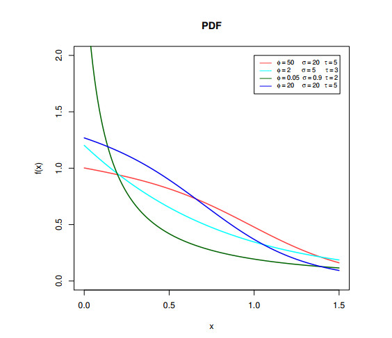
This paper introduces a new extension of the traditional Lomax distribution. The current distribution, which has one scale and two shape parameters, is known as logarithmic transformed Lomax distribution. The hazard rate function of the new distribution based on parameter values, making monotonically decreasing, upside-down and bathtub upside-down shaped. Some properties of the proposed distribution including mixture expansion, moments, entropies, probability weighted moments, order statistics, reversed failure rate and mean past life time are discussed. The distribution parameters are estimated using four frequentist methods: namely, maximum likelihood, least squares, weighted least squares, and maximum product of spacing. The efficiency of the different estimators is compared using a simulation analysis using mean square error. Finally, two real data sets for service times of Aircraft Windshield and survival times of a group of patients given chemotherapy medication are analyzed and compared to some other competing distributions. Based on the results of data analysis, the estimates of minimum and maximum values for the service times of Aircraft Windshield and the survival times of patients given chemotherapy medication are obtained.
Citation: Refah Alotaibi, Hassan Okasha, Hoda Rezk, Abdullah M. Almarashi, Mazen Nassar. On a new flexible Lomax distribution: statistical properties and estimation procedures with applications to engineering and medical data[J]. AIMS Mathematics, 2021, 6(12): 13976-13999. doi: 10.3934/math.2021808
This paper introduces a new extension of the traditional Lomax distribution. The current distribution, which has one scale and two shape parameters, is known as logarithmic transformed Lomax distribution. The hazard rate function of the new distribution based on parameter values, making monotonically decreasing, upside-down and bathtub upside-down shaped. Some properties of the proposed distribution including mixture expansion, moments, entropies, probability weighted moments, order statistics, reversed failure rate and mean past life time are discussed. The distribution parameters are estimated using four frequentist methods: namely, maximum likelihood, least squares, weighted least squares, and maximum product of spacing. The efficiency of the different estimators is compared using a simulation analysis using mean square error. Finally, two real data sets for service times of Aircraft Windshield and survival times of a group of patients given chemotherapy medication are analyzed and compared to some other competing distributions. Based on the results of data analysis, the estimates of minimum and maximum values for the service times of Aircraft Windshield and the survival times of patients given chemotherapy medication are obtained.

| [1] | K. S. Lomax, Business failures: Another example of the analysis of failure data, J. Am. Stat. Assoc., 49 (1954), 847–852. |
| [2] | L. Bain, M. Engelhardt, Introduction to Probability and Mathematical Statistics, Duxbury Press, 1992. |
| [3] | M. E. Ghitany, F. A. Al-Awadhi, L. A. Alkhalfan, Marshall-Olkin extended Lomax distribution and its application to censored data, Commun. Stat. Theory Methods, 36 (2007), 1855–1866. |
| [4] | I. B. Abdul-Moniem, H. F. Abdel-Hameed, On exponentiated Lomax distribution, Int. J. Math. Arch., 3 (2012), 2144–2150. |
| [5] | A. J. Lemonte, G. M. Cordeiro, An extended Lomax distribution, Statistics, 47 (2013), 800–816. |
| [6] | G. M. Cordeiro, E. M. M. Ortega, D. C. C. da Cunha, The Exponentiated Generalized Class of Distributions, J. Data Sci., 11 (2013), 1–27. |
| [7] | M. H. Tahir, G. M. Cordeiro, M. Mansoor, M. Zubair, The Weibull-Lomax distribution: properties and applications, Hacettepe J. Math. Stat., 44 (2015), 461–480. |
| [8] | B. AL-Zahrani, An extended Poisson-Lomax distribution, Adv. Math. Sci. J., 4 (2015), 79–89. |
| [9] | M. Nassar, S. Dey, D. Kumar, Logarithm transformed Lomax distribution with applications, Calcutta Stat. Assoc. Bull., 70 (2018), 122–135. |
| [10] | V. Pappas, K. Adamidis, S. Loukas, A family of lifetime distributions, Int. J. Qual., Stat. Reliab., (2012), 1–6. |
| [11] | B. Al-Zahrani, P. R. D. Marinho, A. A. Fattah, A. H. N. Ahmed, G. M. Cordeiro, The (P-A-L) extended Weibull distribution: a new generalization of the Weibull distribution, Hacettepe J. Math. Stat., 45 (2016), 851–868. |
| [12] | S. Dey, M. Nassar, D. Kumar, Alpha logarithmic transformed family of distributions with applications, Ann. Data Sci., 4 (2017), 457–482. |
| [13] | M. Eltehiwy, Logarithmic inverse Lindley distribution: Model, properties and applications, J. King Saud. Univ. Sci., 32 (2018), 136–144. |
| [14] | I. S. Gradshteyn, I. M. Ryzhik, Tables of Integrals, Series and Products, Seventh Edition, Academic Press, Inc., 2007. |
| [15] | A. Rényi, On measures of entropy and information, In: Berkeley Symposium on Mathematical Statistics and Probability, University of California Press, Berkeley, 1961,547–561. |
| [16] | J. Navarro, M. Franco, J. M. Ruiz, Characterization through moments of the residual life and conditional spacing, Indian J. Stat., Ser. A, 60 (1998), 36–48. |
| [17] | D. N. P. Murthy, M. Xie, R. Jiang, Weibull Models, John Wiley, New York, 2004. |
| [18] | A. Bekker, J. Roux, P. Mostert, A generalization of the compound Rayleigh distribution: using a Bayesian methods on cancer survival times, Commun. Stat. Theory Methods, 29 (2000), 1419–1433. |


Figures(9) / Tables(9)

Refah Alotaibi, Hassan Okasha, Hoda Rezk, Abdullah M. Almarashi, Mazen Nassar. On a new flexible Lomax distribution: statistical properties and estimation procedures with applications to engineering and medical data[J]. AIMS Mathematics, 2021, 6(12): 13976-13999. doi: 10.3934/math.2021808


 DownLoad: