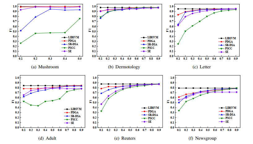
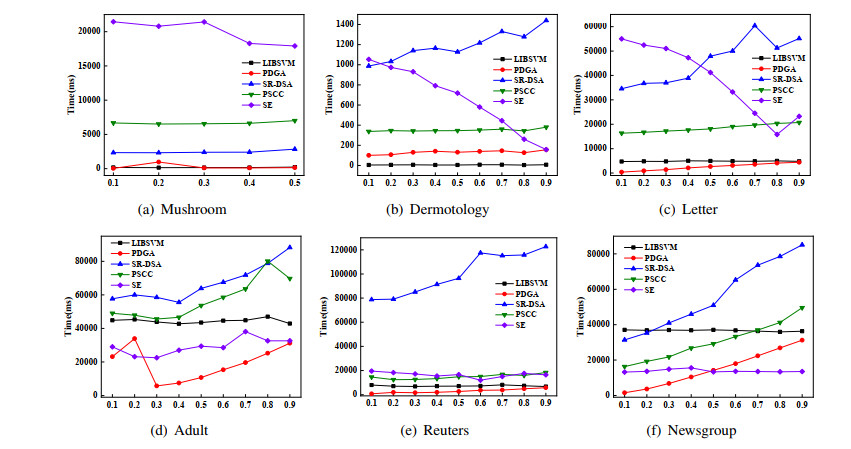
Support vector machine (SVM) is one of the most powerful technologies of machine learning, which has been widely concerned because of its remarkable performance. However, when dealing with the classification problem of large-scale datasets, the high complexity of SVM model leads to low efficiency and become impractical. Due to the sparsity of SVM in the sample space, this paper presents a new parallel data geometry analysis (PDGA) algorithm to reduce the training set of SVM, which helps to improve the efficiency of SVM training. The PDGA introduce Mahalanobis distance to measure the distance from each sample to its centroid. And based on this, proposes a method that can identify non support vectors and outliers at the same time to help remove redundant data. When the training set is further reduced, cosine angle distance analysis method is proposed to determine whether the samples are redundant data, ensure that the valuable data are not removed. Different from the previous data geometry analysis methods, the PDGA algorithm is implemented in parallel, which greatly saving the computational cost. Experimental results on artificial dataset and 6 real datasets show that the algorithm can adapt to different sample distributions. Which significantly reduce the training time and memory requirements without sacrificing the classification accuracy, and its performance is obviously better than the other five competitive algorithms.
Citation: Yunfeng Shi, Shu Lv, Kaibo Shi. A new parallel data geometry analysis algorithm to select training data for support vector machine[J]. AIMS Mathematics, 2021, 6(12): 13931-13953. doi: 10.3934/math.2021806
Support vector machine (SVM) is one of the most powerful technologies of machine learning, which has been widely concerned because of its remarkable performance. However, when dealing with the classification problem of large-scale datasets, the high complexity of SVM model leads to low efficiency and become impractical. Due to the sparsity of SVM in the sample space, this paper presents a new parallel data geometry analysis (PDGA) algorithm to reduce the training set of SVM, which helps to improve the efficiency of SVM training. The PDGA introduce Mahalanobis distance to measure the distance from each sample to its centroid. And based on this, proposes a method that can identify non support vectors and outliers at the same time to help remove redundant data. When the training set is further reduced, cosine angle distance analysis method is proposed to determine whether the samples are redundant data, ensure that the valuable data are not removed. Different from the previous data geometry analysis methods, the PDGA algorithm is implemented in parallel, which greatly saving the computational cost. Experimental results on artificial dataset and 6 real datasets show that the algorithm can adapt to different sample distributions. Which significantly reduce the training time and memory requirements without sacrificing the classification accuracy, and its performance is obviously better than the other five competitive algorithms.

| [1] |
J. Cervantes, F. Garcia-Lamont, L. Rodríguez-Mazahua, A.Lopez, A comprehensive survey on support vector machine classification: Applications, challenges and trends, Neurocomputing, 408 (2020), 189–215. doi: 10.1016/j.neucom.2019.10.118

|
| [2] | Y. Wang, Z. Wang, Q. H. Hu, Y. C. Zhou, H. L. Su, Hierarchical semantic risk minimization for large-scale classification, IEEE T. Cybernetics, 2021, DOI: 10.1109/TCYB.2021.3059631. |
| [3] |
S. H. Alizadeh, A. Hediehloo, N. S. Harzevili, Multi independent latent component extension of naive bayes classifier, Knowl. Based Syst., 213 (2021), 106646. doi: 10.1016/j.knosys.2020.106646
|
| [4] |
L. X. Jiang, C. Q. Li, S. S. Wang, L. G. Zhang, Deep feature weighting for naive bayes and its application to text classification, Eng. Appl. Artif. Intel., 52 (2016), 26–39. doi: 10.1016/j.engappai.2016.02.002
|
| [5] | R. J. Prokop, A. P. Reeves, A survey of moment-based techniques for unoccluded object representation and recognition, CVGIP, 54 (1992), 438–460. |
| [6] |
A. Trabelsi, Z. Elouedi, E. Lefevre, Decision tree classifiers for evidential attribute values and class labels, Fuzzy Set. Syst., 366 (2019), 46–62. doi: 10.1016/j.fss.2018.11.006
|
| [7] | F. C. Pampel, Logistic regression: A primer, Sage publications, 2020. |
| [8] |
P. Skryjomski, B. Krawczyk, A. Cano, Speeding up k-Nearest Neighbors classifier for large-scale multi-label learning on GPUs, Neurocomputing, 354 (2019), 10–19. doi: 10.1016/j.neucom.2018.06.095
|
| [9] |
V. Vapnik, R. Izmailov, Reinforced SVM method and memorization mechanisms, Pattern Recogn., 119 (2021), 108018. doi: 10.1016/j.patcog.2021.108018
|
| [10] | V. N. Vapnik, Statistical learning theory, New York: Wiley, 1998. |
| [11] |
C. J. C. Burges, A tutorial on support vector machines for pattern recognition, Data Min. Knowl. Disc., 2 (1998), 121–167. doi: 10.1023/A:1009715923555
|
| [12] | N. Cristianini, J. Shawe-Taylor, An introduction to support vector machines and other kernel-based learning methods, Cambridge: Cambridge University Press, 2000. |
| [13] |
T. K. Bhowmik, P. Ghanty, A. Roy, S. K. Parui, SVM-based hierarchical architectures for handwritten bangla character recognition, Int. J. Doc. Anal. Recog., 12 (2009), 97–108. doi: 10.1007/s10032-009-0084-x
|
| [14] |
X. P. Liang, L. Zhu, D. S. Huang, Multi-task ranking SVM for image cosegmentation, Neurocomputing, 247 (2017), 126–136. doi: 10.1016/j.neucom.2017.03.060
|
| [15] | Y. S. Chen, Z. H. Lin, X. Zhao, G. Wang, Y. F. Gu, Deep learning-based classification of hyperspectral data, IEEE J.-STARS, 7 (2014), 2094–2107. |
| [16] |
P. Liu, K.-K. R. Choo, L. Z. Wang, F. Huang, SVM or deep learning? A comparative study on remote sensing image classification, Soft Comput., 21 (2017), 7053–7065. doi: 10.1007/s00500-016-2247-2
|
| [17] |
J. Nalepa, M. Kawulok, Adaptive memetic algorithm enhanced with data geometry analysis to select training data for SVMs, Neurocomputing, 185 (2016), 113–132. doi: 10.1016/j.neucom.2015.12.046
|
| [18] |
J. F. Qiu, Q. H. Wu, G. R. Ding, Y. H. Xu, S. Feng, A survey of machine learning for big data processing, EURASIP J. Adv. Sig. Pr., 2016 (2016), 67. doi: 10.1186/s13634-016-0355-x
|
| [19] | T. Joachims, Making large-scale SVM learning practical, Technical Reports, 1998. |
| [20] |
Y. F. Ma, X. Liang, G. Sheng, J. T. Kwok, M. L. Wang, G. S. Li, Noniterative sparse LS-SVM based on globally representative point selection, IEEE T. Neur. Net. Lear., 32 (2021), 788–798. doi: 10.1109/TNNLS.2020.2979466
|
| [21] | J. C. Platt, Sequential minimal optimization: A fast algorithm for training support vector machines, 1998. Available form: https://www.microsoft.com/en-us/research/wp-content/uploads/2016/02/tr-98-14.pdf. |
| [22] | G. Galvan, M. Lapucci, C. J. Lin, M. Sciandrone, A two-level decomposition framework exploiting first and second order information for SVM training problems, J. Mach. Learn. Res., 22 (2021), 1–38. |
| [23] | C. C. Chang, C. J. Lin, LIBSVM: A library for support vector machines, ACM T. Intel. Syst. Tec., 2 (2011), 27. |
| [24] | H. P. Graf, E. Cosatto, L. Bottou, I. Durdanovic, V. Vapnik, Parallel support vector machines: The cascade SVM, In: Advances in Neural Information Processing Systems, 17 (2004), 521–528. |
| [25] | B. L. Lu, K. A. Wang, Y. M. Wen, Comparison of parallel and cascade methods for training support vector machines on large-scale problems, In: Proceedings of the Third International Conference on Machine Learning and Cybernetics, 5 (2004), 3056–3061. |
| [26] | B. Scholkopf, A. J. Smola, Learning with Kernels: Support vector machines, regularization, optimization, and beyond, Cambridge, USA: MIT Press, 2001. |
| [27] |
F. Cheng, J. B. Chen, J. F. Qiu, L. Zhang, A subregion division based multi-objective evolutionary algorithm for SVM training set selection, Neurocomputing, 394 (2020), 70–83 doi: 10.1016/j.neucom.2020.02.028
|
| [28] |
J. Nalepa, M. Kawulok, Selecting training sets for support vector machines: A review, Artif. Intell. Rev., 52 (2019), 857–900. doi: 10.1007/s10462-017-9611-1
|
| [29] |
L. Guo, S. Boukir, Fast data selection for SVM training using ensemble margin, Pattern Recogn. Lett., 51 (2015), 112–119. doi: 10.1016/j.patrec.2014.08.003
|
| [30] | Y. Q. Lin, F. J. Lv, S. H. Zhu, M. Yang, T. Cour, K. Yu, et al., Large-scale image classification: fast feature extraction and SVM training, CVPR, 2011 (2011), 1689–1696. |
| [31] |
A. Lyhyaoui, M. Martinez, I. Mora, M. Vazquez, J. L. Sancho, A. R. Figueiras-Vidal, Sample selection via clustering to construct support vector-like classifiers, IEEE T. Neural Networ., 10 (1999), 1474–1481. doi: 10.1109/72.809092
|
| [32] |
G. W. Gates, The reduced nearest neighbor rule, IEEE T. Inform. Theory, 18 (1972), 431–433. doi: 10.1109/TIT.1972.1054809
|
| [33] | M. Kawulok, J. Nalepa, Support vector machines training data selection using a genetic algorithm, In: Structural, dyntactic, and dtatistical pattern recognition, Springer, Berlin, Heidelberg, 2012. |
| [34] |
D. R. Musicant, A. Feinberg, Active set support vector regression, IEEE T. Neural Networ., 15 (2004), 268–275. doi: 10.1109/TNN.2004.824259
|
| [35] |
F. Alamdar, S. Ghane, A. Amiri, On-line twin independent support vector machines, Neurocomputing, 186 (2016), 8–21. doi: 10.1016/j.neucom.2015.12.062
|
| [36] |
D. R. Wilson, T. R. Martinez, Reduction techniques for instance-based learning algorithms, Mach. Learn., 38 (2000), 257–286. doi: 10.1023/A:1007626913721
|
| [37] |
M. Ryu, K. Lee, Selection of support vector candidates using relative support distance for sustainability in large-scale support vector machines, Appl. Sci., 10 (2020), 6979. doi: 10.3390/app10196979
|
| [38] | J. Balc{á}zar, Y. Dai, O. Watanabe, A random sampling technique for training support vector machines, In: Algorithmic learning theory, 2001,119–134. |
| [39] |
F. Zhu, J. Yang, N. Ye, C. Gao, G. B. Li, T. M. Yin, Neighbors' distribution property and sample reduction for support vector machines, Appl. Soft. Comput., 16 (2014), 201–209. doi: 10.1016/j.asoc.2013.12.009
|
| [40] |
X. O. Li, J. Cervantes, W. Yu, Fast classification for large data sets via random selection clustering and support vector machines, Intell. Data Anal., 16 (2012), 897–914. doi: 10.3233/IDA-2012-00558
|
| [41] | S. Abe, T. Inoue, Fast training of support vector machines by extracting boundary data, In: International Conference on Artificial Neural Networks, Springer, Berlin, Heidelberg, 2001,308–313. |
| [42] |
P. Hart, The condensed nearest neighbor rule (corresp.), IEEE T. Inform. Theory, 14 (1968), 515–516. doi: 10.1109/TIT.1968.1054155
|
| [43] |
H. Shin, S. Cho, Neighborhood property–based pattern selection for support vector machines, Neural Comput., 19 (2007), 816–855. doi: 10.1162/neco.2007.19.3.816
|
| [44] | J. T. Xia, M. Y. He, Y. Y. Wang, Y. Feng, A fast training algorithm for support vector machine via boundary sample selection, In: International Conference on Neural Networks and Signal Processing, 2003, 20–22. |
| [45] | R. Pighetti, D. Pallez, F. Precioso, Improving SVM training sample selection using multi-objective evolutionary algorithm and LSH, In: 2015 IEEE Symposium Series on Computational Intelligence, 2015, 1383–1390. |
| [46] | J. Kremer, K. S. Pedersen, C. Igel, Active learning with support vector machines, In: Wiley Interdisciplinary Reviews: Data Mining and Knowledge Discovery, 4 (2014), 313–326. |
| [47] | R. Wang, S. Kwong, Sample selection based on maximum entropy for support vector machines, In: 2010 International Conference on Machine Learning and Cybernetics, 2010, 1390–1395. |
| [48] |
W. J. Wang, Z. B. Xu, A heuristic training for support vector regression, Neurocomputing, 61 (2004), 259–275. doi: 10.1016/j.neucom.2003.11.012
|
| [49] |
D. F. Wang, L. Shi, Selecting valuable training samples for SVMs via data structure analysis, Neurocomputing, 71 (2008), 2772–2781. doi: 10.1016/j.neucom.2007.09.008
|
| [50] |
C. Liu, W. Y. Wang, M. Wang, F. M. Lv, M. Konan, An efficient instance selection algorithm to reconstruct training set for support vector machine, Knowl. Based Syst., 116 (2017), 58–73. doi: 10.1016/j.knosys.2016.10.031
|
| [51] |
C. Leys, O. Klein, Y. Dominicy, C. Ley, Detecting multivariate outliers: Use a robust variant of the mahalanobis distance, J. Exp. Soc. Psychol., 74 (2018), 150–156. doi: 10.1016/j.jesp.2017.09.011
|
| [52] | J. A. K. Suykens, T. Van Gestel, J. De Brabanter, B. De Moor, J. Vandewalle, Least squares support vector machines, World Scientific, 2002. |
| [53] | L. Yu, W. D. Yi, D. K. He, y. Lin, Fast reduction for large-scale training data set, J. Southwest Jiaotong Univ., 42 (2007), 460–468. |
Figures(10) / Tables(4)

Yunfeng Shi, Shu Lv, Kaibo Shi. A new parallel data geometry analysis algorithm to select training data for support vector machine[J]. AIMS Mathematics, 2021, 6(12): 13931-13953. doi: 10.3934/math.2021806


 DownLoad: