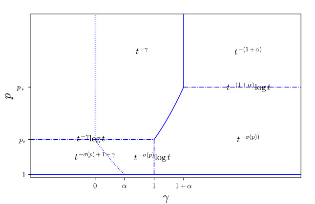
We study the decay/growth rates in all Lp norms of solutions to an inhomogeneous nonlocal heat equation in RN involving a Caputo α-time derivative and a power β of the Laplacian when the dimension is large, N>4β. Rates depend strongly on the space-time scale and on the time behavior of the spatial L1 norm of the forcing term.
Citation: Carmen Cortázar, Fernando Quirós, Noemí Wolanski. Decay/growth rates for inhomogeneous heat equations with memory. The case of large dimensions[J]. Mathematics in Engineering, 2022, 4(3): 1-17. doi: 10.3934/mine.2022022
[1] | Hoai-Minh Nguyen, Tu Nguyen . Approximate cloaking for the heat equation via transformation optics. Mathematics in Engineering, 2019, 1(4): 775-788. doi: 10.3934/mine.2019.4.775 |
[2] | Federico Cluni, Vittorio Gusella, Dimitri Mugnai, Edoardo Proietti Lippi, Patrizia Pucci . A mixed operator approach to peridynamics. Mathematics in Engineering, 2023, 5(5): 1-22. doi: 10.3934/mine.2023082 |
[3] | Franco Flandoli, Eliseo Luongo . Heat diffusion in a channel under white noise modeling of turbulence. Mathematics in Engineering, 2022, 4(4): 1-21. doi: 10.3934/mine.2022034 |
[4] | Ko-Shin Chen, Cyrill Muratov, Xiaodong Yan . Layered solutions for a nonlocal Ginzburg-Landau model with periodic modulation. Mathematics in Engineering, 2023, 5(5): 1-52. doi: 10.3934/mine.2023090 |
[5] | Giacomo Ascione, Daniele Castorina, Giovanni Catino, Carlo Mantegazza . A matrix Harnack inequality for semilinear heat equations. Mathematics in Engineering, 2023, 5(1): 1-15. doi: 10.3934/mine.2023003 |
[6] | Daniele Castorina, Giovanni Catino, Carlo Mantegazza . A triviality result for semilinear parabolic equations. Mathematics in Engineering, 2022, 4(1): 1-15. doi: 10.3934/mine.2022002 |
[7] | Massimiliano Giona, Luigi Pucci . Hyperbolic heat/mass transport and stochastic modelling - Three simple problems. Mathematics in Engineering, 2019, 1(2): 224-251. doi: 10.3934/mine.2019.2.224 |
[8] | José Antonio Vélez-Pérez, Panayotis Panayotaros . Wannier functions and discrete NLS equations for nematicons. Mathematics in Engineering, 2019, 1(2): 309-326. doi: 10.3934/mine.2019.2.309 |
[9] | Gabriel B. Apolinário, Laurent Chevillard . Space-time statistics of a linear dynamical energy cascade model. Mathematics in Engineering, 2023, 5(2): 1-23. doi: 10.3934/mine.2023025 |
[10] | Masashi Misawa, Kenta Nakamura, Yoshihiko Yamaura . A volume constraint problem for the nonlocal doubly nonlinear parabolic equation. Mathematics in Engineering, 2023, 5(6): 1-26. doi: 10.3934/mine.2023098 |
We study the decay/growth rates in all Lp norms of solutions to an inhomogeneous nonlocal heat equation in RN involving a Caputo α-time derivative and a power β of the Laplacian when the dimension is large, N>4β. Rates depend strongly on the space-time scale and on the time behavior of the spatial L1 norm of the forcing term.
Dedicated to the memory of our good friend Ireneo Peral, whose enthusiasm for mathematics and life will always be a model for us.
This paper is part of a project intending to give a precise description (decay/growth rates and profiles) of the large-time behavior of solutions to the Cauchy problem
∂αtu+(−Δ)βu=fin Q:=RN×(0,∞),u(⋅,0)=u0in RN, | (1.1) |
where u0 and f(⋅,t) belong to L1(RN). Here, ∂αt, α∈(0,1), denotes the so-called Caputo α-derivative, introduced independently by many authors using different points of view, see for instance [2,11,13,15,17,20], defined for smooth functions by
∂αtu(x,t)=1Γ(1−α)∂t∫t0u(x,s)−u(x,0)(t−s)αds, |
and (−Δ)β, β∈(0,1], is the usual β power of the Laplacian, defined for smooth functions by (−Δ)β=F−1(|⋅|2βF), where F stands for Fourier transform; see for instance [21].
Fully nonlocal heat equations like (1.1), nonlocal both in space and time, are useful to model situations with long-range interactions and memory effects, and have been proposed for example to describe plasma transport [8,9]; see also [3,4,18,22] for further models that use such equations.
When the forcing term f is trivial, a complete description of the large-time behavior of (1.1) was recently given in [5,6]; see also [16]. Hence, since the problem is linear, it only remains to study the case with trivial initial datum, namely
∂αtu+(−Δ)βu=fin Q,u(⋅,0)=0in RN. | (1.2) |
This task is by far more involved, and this paper represents a first step towards its completion. It is devoted to the obtention of (sharp) decay/growth rates of solutions to (1.2) when the forcing term satisfies
‖f(⋅,t)‖L1(RN)≤C(1+t)γfor some γ∈R | (1.3) |
and the spatial dimension is large, N>4β. This already involves critical phenomena depending on the values of p and γ. If 1≤N≤4β, additional critical phenomena associated to the dimension appear, that make the analysis somewhat different. This case is considered in [7]. Notice that we are allowing γ to take negative values, so that ‖f(⋅,t)‖L1(RN) may grow with time.
If f(⋅,t)∈L1(RN) for all t≥0 and |Ff(ξ,t)|≤C|g(ξ)| for some function g such that
(1+|⋅|2β)g(⋅)∈L1(RN), |
then problem (1.2) has a unique bounded classical solution given by Duhamel's type formula
u(x,t)=∫t0∫RNY(x−y,t−s)f(y,s)dyds, | (1.4) |
with Y=∂1−αtZ, where Z is the solution to (1.2) with f≡0 having a Dirac mass as initial datum; see [12,16]. If we only assume f∈L∞loc([0,∞):L1(RN)), the function u in (1.4) is still well defined, but it is not in general a classical solution to (1.2). Nevertheless, it is a solution in a generalized sense [14,16]. In this paper we will always deal with solutions of this kind, given by (1.4), which are denoted in the literature as mild solutions [16,19].
Notation. As is common in asymptotic analysis, g≍h will mean that there are constants ν,μ>0 such that νh≤g≤μh.
Since the mild solution is given by the convolution in space and time of the forcing term f with the kernel Y, having good estimates for the latter will be essential for the analysis. Such estimates were obtained in [16], and are recalled next.
The kernel Y has a self-similar form,
Y(x,t)=t−σ∗G(ξ),ξ=xt−θ,σ∗:=1−α+Nθ,θ:=α2β. | (1.5) |
Its profile G is positive, radially symmetric and smooth outside the origin, and if N>4β satisfies the sharp estimates
G(ξ)≍|ξ|4β−N,|ξ|≤1, β∈(0,1], | (1.6) |
G(ξ)≍|ξ|(N−2)(α−1)(2−α)exp(−σ|ξ|22−α),|ξ|≥1, β=1, | (1.7) |
G(ξ)≍|ξ|−(N+2β),|ξ|≥1, β∈(0,1). | (1.8) |
In particular, we have the global bound
0≤Y(x,t)≤Ct−(1+α)|x|4β−Nin Q,β∈(0,1], | (1.9) |
and, since |ξ|(N−2)(α−1)(2−α)exp(−σ|ξ|22−α)≤Cν|ξ|−(N+2β) if |ξ|≥ν, also the exterior bound
0≤Y(x,t)≤Cνt2α−1|x|−(N+2β)if |x|≥νtθ, t>0,β∈(0,1]. | (1.10) |
Notice that Y(⋅,t)∈Lp(RN) if and only if p∈[1,p∗), where p∗:=N/(N−4β). Moreover,
‖Y(⋅,t)‖Lp(RN)=Ct−σ(p),σ(p):=1−α+Nθ(1−1p),for all t>0,if p∈[1,p∗). | (1.11) |
Therefore, Y∈L1loc([0,∞):Lp(RN)) if and only if p∈[1,pc), where pc:=N/(N−2β). Since the mild solution is given by a convolution of f with Y both in space and time, the threshold value that will mark the border between subcritical and supercritical behaviors will be pc, and not p∗. In particular, condition (1.3) guarantees that u(⋅,t)∈Lp(RN) for p∈[1,pc), but not for p≥pc. Hence, in order to deal with supercritical exponents p≥pc we need some extra assumption on the spatial behavior of the forcing term. In the present paper we will use two different such extra hypotheses, the pointwise condition
|f(x,t)|≤C|x|−N(1+t)−γfor |x| large, | (1.12) |
and the integral condition
‖f(⋅,t)‖Lq(RN)≤C(1+t)−γfor some q>qc(p):=N2β+Np. | (1.13) |
We do not claim that these conditions are optimal; but they are not too restrictive, and are easy enough to keep the proofs simple.
The only precedent is given in [16], where the authors study the problem in the integrable in time case γ>1 and prove, for all p∈[1,∞] if 1≤N<4β, and for p∈[1,pc) if N≥4β, that
limt→∞tσ(p)‖u(⋅,t)−M∞Y(⋅,t)‖Lp(RN)=0,where M∞:=∫∞0∫RNf(x,t)dxdt<∞. | (1.14) |
In particular, using (1.11) we get the sharp estimate
‖u(⋅,t)‖Lp(RN)≤Ct−σ(p). |
This result is also valid for the local case, α=1, β=1; see for instance [1,10] for the case p=1. In this special situation Y=Z is the well-known fundamental solution of the heat equation, whose profile does not have a spatial singularity and belongs to all Lp spaces.
An analogous convergence result is definitely not possible for α∈(0,1) if p≥p∗, since Y(⋅,t)∉Lp(RN) in that case, or if γ≤1. Moreover, even in the subcritical range (1.14) only gives a sharp rate and a nontrivial limit profile in the diffusive scale |x|≍tθ; see below. Hence we need a different approach.
As we will see, it turns out that, in contrast with the local case, and due to the effect of memory, the decay/growth rates are not the same in different space-time scales. Moreover, the scale that determines the dominant rate depends on the value of the exponent p. Our strategy will consist in tackling this difficulty directly by studying separately the rates in exterior regions, |x|≥νtθ with ν>0, compact sets or intermediate regions |x|≍g(t) with g(t)→∞ and g(t)=o(tθ). We already found this phenomenon for the Cauchy problem, (1.1) with f≡0, where the decay rate was O(t−α) in compact sets and O(t−Nθ(1−1p)) in exterior regions; see [5,6].
Our first result concerns exterior regions.
Theorem 1.1 (Exterior regions). Let f satisfy (1.3) and also (1.12) if p≥pc. Let u be the mild solution to (1.2). For all ν>0 there is a constant C such that
‖u(⋅,t)‖Lp({|x|≥νtθ})≤C{t−σ(p)+1−γ,γ<1,t−σ(p)logt,γ=1,t−σ(p),γ>1. | (1.15) |
These estimates are sharp.
For p∈[1,pc) and γ>1 the result follows from (1.14), showing that the behavior in this regions dominates the global behavior in the subcritical case.
We now turn to the behavior in compact sets which, due to the effect of memory, will dominate the global behavior for large values of p.
Theorem 1.2 (Compact sets). Let f satisfy (1.3). If p≥pc, assume also (1.13) with γ as in (1.3). Let u be the mild solution to (1.2). For every compact set K there exists a constant C such that
‖u(⋅,t)‖Lp(K)≤C{t−γ,γ≤1+α,t−(1+α),γ≥1+α. | (1.16) |
These estimates are sharp.
Remark. Note that qc(pc)=1.
As expected, the rates in intermediate regions, between compact sets and exterior regions, are intermediate between the ones in such scales.
Theorem 1.3 (Intermediate regions). Let f satisfy (1.3) and also (1.12) if p≥pc. Let g(t)→∞ be such that g(t)=o(tθ). Let u be the mild solution to (1.2). For all 0<ν<μ<∞ there exists a constant C such that
‖u(⋅,t)‖Lp({ν≤|x|/g(t)≤μ})≤Cg(t)2β−N(1−1p){t−γ,γ<1,max{t−1,t−(1+α)g(t)2βlogt},γ=1,max{t−γ,t−(1+α)g(t)2β},γ>1. | (1.17) |
These estimates are sharp.
We also obtain results that connect the behaviors in compact sets and exterior regions, thus getting the (global) decay rate in Lp(RN).
Theorem 1.4 (Global results). Assume (1.3), and also (1.12) and (1.13) with γ as in (1.3) if p≥pc. Let u be the mild solution to (1.2). There is a constant C such that
‖u(⋅,t)‖Lp(RN)≤C{t−σ(p)+1−γ,γ<1,t−σ(p)logt,γ=1,p∈[1,pc),t−σ(p),γ>1,t−γlogt,γ≤1,p=pc,t−1,γ>1,t−γ,γ≤σ(p),p∈(pc,p∗),t−σ(p),γ≥σ(p),t−γ,γ<1+α,p=p∗,t−(1+α)logt,γ≥1+α,t−γ,γ≤1+α,p>p∗,t−(1+α),γ≥1+α; |
see Figure 1. These estimates are sharp.
Notice that the borderline separating decay and growth is γ=0 only for p≥pc. For p∈[1,pc) the frontier is given by
γ=1−σ(p); |
see the dotted line in Figure 1. For p=1 this corresponds to γ=α. An informal explanation for this fact can be found in formula (1.4). We are integrating in time, but Y(x,t)=∂1−αtZ(x,t). Hence, it is like if we were integrating α times in time. As for the behavior for the borderline γ, in general there is neither growth nor decay. The exception is the case p=pc, γ=0, in which there is a slow logarithmic growth.
Another remarkable fact is that the rates depend on γ not only in the non-integrable case γ≤1, which might have been expected, but also in part of the region γ∈[1,1+α) if p is supercritical.
In this section we prove Theorem 1.1, which gives the behavior of all Lp norms of the mild solution u to (1.2) in exterior regions, {(x,t)∈Q:|x|≥νtθ}, ν>0.
Proof of Theorem 1.1. The starting point is Duhamel's type formula (1.4). If p∈[1,pc), then Y(⋅,t) belongs to Lp(RN). Therefore, using (1.3) and (1.11),
‖u(⋅,t)‖Lp(RN)≤∫t0‖Y(⋅,t−s)‖Lp(RN)‖f(⋅,s)‖L1(RN)ds≤C∫t0(t−s)−σ(p)(1+s)−γds≤Ct−σ(p)∫t20(1+s)−γds+Ct−γ∫tt2(t−s)−σ(p)ds≤Ct−σ(p)∫t20(1+s)−γds+Ct−σ(p)+1−γ. |
Integration of ∫t20(1+s)−γds gives the result.
We turn now our attention to the case p≥pc, for which we assume also the decay condition (1.12). We have |u|≤I+II, where
I(x,t)=∫t0∫{|y|<|x|2}Y(x−y,t−s)|f(y,s)|dyds,II(x,t)=∫t0∫{|y|>|x|2}Y(x−y,t−s)|f(y,s)|dyds. |
We start by estimating I. Notice that if |y|<|x|/2, then |x−y|>|x|/2. Thus, if moreover |x|≥νtθ, there holds that |x−y|(t−s)−θ>ν/2. Hence, the bound (1.10) yields
Y(x−y,t−s)≤C(t−s)2α−1|x−y|−(N+2β)≤C(t−s)2α−1|x|−(N+2β). |
Using also (1.3) we arrive at I(x,t)≤C|x|−(N+2β)∫t0(t−s)2α−1(1+s)−γds, and therefore
‖I(⋅,t)‖Lp({|x|≥νtθ})≤Ct−σ(p)+1−2α(∫t20(1+s)−γ(t−s)2α−1ds+∫tt2(1+s)−γ(t−s)2α−1ds)≤Ct−σ(p)∫t20(1+s)−γds+Ct−σ(p)+1−γ−2α∫tt2(t−s)2α−1ds≤Ct−σ(p)∫t20(1+s)−γds+Ct−σ(p)+1−γ, |
and the desired bound for I follows.
Now we turn to II. We choose ε∈(0,1/2). Given x∈RN, t>0, s∈(0,t), we denote B(x,t,s)={y∈RN:|x−y|<|x|ε(t−s)θ(1−ε)}. Note that for |x|>νtθ and y∈(B(x,t,s))c we have |x−y|(t−s)−θ>νε. Therefore, using the estimates (1.9)–(1.10), we have II≤II1+II2, with
II1(x,t)=C∫t0∫{|y|>|x|2}∩B(x,t,s)(t−s)−(1+α)|x−y|4β−N|f(y,s)|dyds,II2(x,t)=C∫t0∫{|y|>|x|2}∩(B(x,t,s))c(t−s)2α−1|x−y|−(N+2β)|f(y,s)|dyds. |
We have, using the decay condition (1.12),
II1(x,t)≤C∫t0∫{|y|>|x|2}∩B(x,t,s)|y|−N(1+s)−γ(t−s)−(1+α)|x−y|4β−Ndyds≤C|x|−N∫t0(1+s)−γ(t−s)−(1+α)∫B(x,t,s)|x−y|4β−Ndyds=C|x|4βε−N∫t0(1+s)−γ(t−s)α(1−2ε)−1ds. |
Since p≥pc and ε∈(0,1/2), we have (N−4βε)p>N, and hence
‖II1(⋅,t)‖Lp({|x|>νtθ})=Ct−σ(p)+1−α(1−2ε)∫t0(1+s)−γ(t−s)α(1−2ε)−1ds≤Ct−σ(p)∫t20(1+s)−γds+Ct−σ(p)+1−γ, |
and integration gives the bound in (1.15) for this term.
Finally, since |x−y|≥|x|ε(t−s)θ(1−ε) in (B(x,t,s))c, using the condition (1.3) on f,
II2(x,t)≤C|x|−(N+2β)ε∫t0(1+s)−γ(t−s)−σ∗+θ(N+2β)εds, |
so that
‖II2(⋅,t)‖Lp({|x|>νtθ})≤CtNθp−θ(N+2β)ε∫t0(1+s)−γ(t−s)−σ∗+θ(N+2β)εds≤Ct−σ(p)∫t20(1+s)−γds+Ct−σ(p)+1−γ. |
Now, integration gives the bound.
In order to check that the bound in (1.15) is sharp we choose f(x,t)=(1+t)−γχB1(x). If t is large, |y|<1 and |x|>νtθ, then |y|<|x|/2. Hence, |x|/2<|x−y|<3|x|/2, so that, assuming also that |x|<μtθ and 0<s<t/2,
ν2≤|x|2tθ≤|x−y|(t−s)θ≤3μ2(tt−s)θ≤C. |
Thus, since the profile G of Y is positive, under these conditions Y(x−y,t−s)≥C(t−s)−σ∗ for some constant C>0, see (1.5), and therefore,
u(x,t)≥C∫t20(1+s)−γ(t−s)−σ∗ds≥Ct−σ∗∫t20(1+s)−γds. |
Thus,
‖u(⋅,t)‖Lp({|x|>νtθ})≥‖u(⋅,t)‖Lp({μ>|x|/tθ>ν})≥Ct−σ∗|{νtθ<|x|<μtθ}|1/p∫t20(1+s)−γds=Ct−σ(p)∫t20(1+s)−γds, |
which implies the desired lower bound.
In this section we prove Theorem 1.2, which gives the large-time behavior of the Lp norms of the mild solution to (1.3) in compact sets K.
Proof of Theorem 1.2. Let t≥1. We have |u|≤I+II, where
I(x,t)=∫t−10∫RNY(x−y,t−s)|f(y,s)|dyds,II(x,t)=∫tt−1∫RNY(x−y,t−s)|f(y,s)|dyds. |
Using the global bound (1.9) for Y we get
I(x,t)≤C∫t−10(t−s)−(1+α)∫RN|x−y|4β−N|f(y,s)|dyds≤C∫t−10(t−s)−(1+α)∫{|x−y|<1}|x−y|4β−N|f(y,s)|dyds+C∫t−10(t−s)−(1+α)∫{|x−y|>1}|f(y,s)|dyds. |
Let q=1 if p∈[1,pc), q>qc(p) as in (1.13) if p≥pc. Let r satisfy 1+1p=1q+1r. Then r∈[1,pc), and in particular r∈[1,p∗). Thus, for all t≥2 we have
‖I(⋅,t)‖Lp(K)≤C∫t−10(t−s)−(1+α)‖f(⋅,s)‖Lq(K+B1)(∫B1|z|(4β−N)rdz)1/rds+C|K|1/p∫t−10(t−s)−(1+α)‖f(⋅,s)‖L1(RN)ds≤C∫t−10(1+s)−γ(t−s)−(1+α)ds≤Ct−(1+α)∫t20(1+s)−γds+Ct−γ∫t−1t2(t−s)−(1+α)ds≤Ct−γ+C{t−(γ+α),γ<1,t−(1+α)logt,γ=1,t−(1+α),γ>1, |
which implies that ‖I(⋅,t)‖Lp(K)≤Ct−min{γ,1+α}.
In order to bound II we take r∈[1,pc) as before. Then, using (1.11) we get
‖II(⋅,t)‖Lp(K)≤C∫tt−1‖f(⋅,s)‖Lq(RN)(t−s)α−1−Nθ(1−1r)ds≤C∫tt−1(1+s)−γ(t−s)α−1−Nθ(1−1r)ds≤Ct−γ∫10τα−1−Nθ(1−1r)dτ=Ct−γ, |
which combined with the estimate for I yields the result.
In order to prove that estimate (1.16) is sharp we consider f(x,t)=(1+t)−γχK+B1(x), where K is any compact set with measure different from 0. We have
u(x,t)≥∫t−10(1+s)−γ∫K+B1Y(x−y,t−s)dyds. |
If x∈K and |x−y|<1, then y∈K+B1. Notice that |x−y|<1 and s<t−1 imply that |x−y|(t−s)−θ≤1. Therefore, using the self-similar form (1.5) of Y and the bound from below (1.6) for the profile G, for all x∈K we have
u(x,t)≥C∫t−10(1+s)−γ(t−s)−(1+α)∫{|x−y|<1}|x−y|4β−Ndyds=C∫t−10(1+s)−γ(t−s)−(1+α)ds |
for some constant C>0. Thus, no matter the value of γ, for all x∈K and t large enough,
u(x,t)≥Ct−γ∫t−1t2(t−s)−(1+α)ds=Ct−γ∫t21τ−(1+α)dτ≥Ct−γ, |
while if γ>1, then
u(x,t)≥C∫t20(1+s)−γ(t−s)−(1+α)ds≥Ct−(1+α)∫t20(1+s)−γds≥Ct−(1+α), |
so that ‖u(⋅,t)‖Lp(K)≥Ct−min{γ,1+α}.
In this section we study the large-time behavior of the Lp norms of the mild solution to (1.3) in regions where |x|≍g(t) with g(t)→∞ such that g(t)=o(tθ), which is the content of Theorem 1.3.
Proof of Theorem 1.3. We have |u|≤I+II, where
I(x,t)=∫t0∫{|y|>|x|2}|f(x−y,t−s)|Y(y,s)dyds,II(x,t)=∫t0∫{|y|<|x|2}|f(x−y,t−s)|Y(y,s)dyds. | (4.1) |
To estimate I we decompose it as I=I1+I2+I3, where
I1(x,t)=∫(|x|2)1/θ0∫{|y|>|x|2}|f(x−y,t−s)|Y(y,s)dyds,I2(x,t)=∫t2(|x|2)1/θ∫{|y|>|x|2}|f(x−y,t−s)|Y(y,s)dyds,I3(x,t)=∫tt2∫{|y|>|x|2}|f(x−y,t−s)|Y(y,s)dyds. | (4.2) |
If 0<sθ<|x|/2<|y|, then |y|s−θ≥1. Therefore, using (1.10) and condition (1.3), if |x|<μg(t) with g(t)=o(tθ) we have
I1(x,t)≤C|x|−(N+2β)∫(|x|2)1/θ0s2α−1(1+t−s)−γds≤C|x|2β−Nt−γ. | (4.3) |
Thus, ‖I1(⋅,t)‖Lp({ν<|x|/g(t)<μ})≤Ct−γg(t)2β−N(1−1p).
As for I2 and I3, using the global bound (1.9) for Y and condition (1.3),
I2(x,t)≤C|x|4β−N∫t2(|x|2)1/θ(1+t−s)−γs−(1+α)ds≤C|x|4β−Nt−γ∫t2(|x|2)1/θs−(1+α)ds≤C|x|2β−Nt−γ,I3(x,t)≤C|x|4β−Nt−(1+α)∫t20(1+τ)−γdτ. | (4.4) |
Therefore,
‖I2(⋅,t)‖Lp({ν<|x|/g(t)<μ})≤Ct−γg(t)2β−N(1−1p),‖I3(⋅,t)‖Lp({ν<|x|/g(t)<μ})≤Cg(t)4β−N(1−1p){t−(γ+α),γ<1,t−(1+α)logt,γ=1,t−(1+α),γ>1. |
Now we turn to II. We decompose it as II≤II1+II2, where
II1(x,t)=C∫t20∫{|y|<|x|2}|f(x−y,t−s)|Y(y,s)dyds,II2(x,t)=C∫tt2∫{|y|<|x|2}|f(x−y,t−s)|Y(y,s)dyds. | (4.5) |
We start with the subcritical case p∈[1,pc). Notice that if sθ<|y|, then |y|s−θ≥1. Moreover, if |x|=o(tθ), then (|x|/2)1/θ=o(t), and hence (|x|/2)1/θ<t/2 if t is large. Therefore, using the bounds (1.9) and (1.10), we have II1≤II11+II12, where
II11(x,t)=C∫(|x|2)1/θ0∫{sθ<|y|<|x|2}|f(x−y,t−s)|s2α−1|y|−(N+2β)dyds,II12(x,t)=C∫t20∫{|y|<min{|x|2,sθ}}|f(x−y,t−s)|s−(1+α)|y|4β−Ndyds. |
Using condition (1.3), and remembering that g(t)=o(tθ),
‖II11(⋅,t)‖Lp({ν<|x|/g(t)<μ})≤C∫(μ2g(t))1/θ0‖f(⋅,t−s)‖L1(RN)s2α−1(∫{|y|>sθ}|y|−(N+2β)pdy)1/pds≤C∫(μ2g(t))1/θ0(1+t−s)−γs−σ(p)ds≤Ct−γg(t)2β−N(1−1p),‖II12(⋅,t)‖Lp({ν<|x|/g(t)<μ})≤C∫(μ2g(t))1/θ0‖f(⋅,t−s)‖L1(RN)s−(1+α)(∫{|y|<sθ}|y|(4β−N)pdy)1/pds+C∫t2(μ2g(t))1/θ‖f(⋅,t−s)‖L1(RN)s−(1+α)(∫{|y|<μ2g(t)}|y|(4β−N)pdy)1/pds≤Ct−γ∫(μ2g(t))1/θ0s−σ(p)ds+Cg(t)4β−N(1−1p)t−γ∫t2(μ2g(t))1/θs−(1+α)ds≤Ct−γg(t)2β−N(1−1p). |
On the other hand, from the global bound (1.9),
II2(x,t)=C∫tt2∫{|y|<|x|2}|f(x−y,t−s)|s−(1+α)|y|4β−Ndyds, |
and therefore, thanks to condition (1.3),
‖II2(⋅,t)‖Lp({ν<|x|/g(t)<μ})≤∫tt2‖f(⋅,t−s)‖L1(RN)s−(1+α)(∫{|y|<μ2g(t)}|y|(4β−N)pdy)1/pds≤Cg(t)4β−N(1−1p)t−(1+α)∫t20(1+τ)−γdτ≤Cg(t)4β−N(1−1p){t−(γ+α),γ<1,t−(1+α)logt,γ=1,t−(1+α),γ>1. |
Let now p≥pc. Since |x−y|≥|x|/2≥νg(t)/2→∞ as t→∞, then, thanks to assumption (1.12), we have that |f(x−y,t−s)|≤C|x|−N(1+t−s)−γ for all t large. Hence,
II11(x,t)≤C|x|−N∫(|x|2)1/θ0(1+t−s)−γs2α−1∫{|y|>sθ}|y|−(N+2β)dyds=C|x|−N∫(|x|2)1/θ0(1+t−s)−γsα−1ds≤C|x|−Nt−γ∫(|x|2)1/θ0sα−1ds=C|x|2β−Nt−γ,II12(x,t)≤C|x|−N(∫(|x|2)1/θ0(1+t−s)−γs−(1+α)∫{|y|<sθ}|y|4β−Ndyds+∫t2(|x|2)1/θ(1+t−s)−γs−(1+α)∫{|y|<|x|2}|y|4β−Ndyds)≤C|x|−Nt−γ∫(|x|2)1/θ0sα−1ds+C|x|4β−Nt−γ∫t2(|x|2)1/θs−(1+α)ds≤C|x|2β−Nt−γ. |
Therefore, ‖II1(⋅,t)‖Lp({ν<|x|/g(t)<μ})≤Ct−γg(t)2β−N(1−1p) also when p≥pc.
As for II2, also when p≥pc, since |y|<|x|/2 implies |x−y|>|x|/2, using the global estimate (1.9) and the decay condition (1.12),
II2(x,t)≤C|x|−N∫tt2(1+t−s)−γs−(1+α)∫{|y|<|x|2}|y|4β−Ndyds≤C|x|4β−Nt−(1+α)∫t20(1+τ)−γdτ≤C|x|4β−N{t−(γ+α),γ<1,t−(1+α)logt,γ=1,t−(1+α),γ>1, |
and hence
‖II2(⋅,t)‖Lp({ν<|x|/g(t)<μ})≤Cg(t)4β−N(1−1p){t−(γ+α),γ<1,t−(1+α)logt,γ=1,t−(1+α),γ>1. |
Estimate (1.17) follows from the above bounds and the fact that g(t)=o(tθ).
To end the proof we have to check that (1.17) is sharp. To this aim we take f(x,t)=(1+t)−γχB1(x). Let t be large enough so that g(t)>2/ν. If νg(t)<|x|<μg(t) and |x−y|<1,
ν2g(t)<|x|2<|x|−ν2g(t)<|x|−1<|y|<|x|+1<|x|+ν2g(t)<2|x|<2μg(t). | (4.6) |
Under these assumptions, if s∈(0,(νg(t)/2)1/θ), then |y|s−θ≥|y|/(νg(t)/2)≥1. Therefore, if g(t)=o(tθ), using (1.5) and the estimates from below in (1.7)–(1.8), and performing the change of variables s=τg(t)1/θ, we arrive at
u(x,t)≥∫(ν2g(t))1/θ0∫{|x−y|<1}(1+t−s)−γY(y,s)dyds≥Ct−γ∫(ν2g(t))1/θ0s−σ∗e−c(g(t)s−θ)22−αds=Ct−γg(t)2β−N∫(ν2)1/θ0τ−σ∗e−cτ−αβ(2−α)dτ=Ct−γg(t)2β−N. |
Therefore,
‖u(x,t)‖Lp({ν<|x|/g(t)<μ})≥Ct−γg(t)2β−N(1−1p). | (4.7) |
On the other hand, under the assumptions leading to (4.6), if moreover s∈(t/2,t) and t is large enough, we have |y|<2μg(t)<(t/2)θ<sθ. Thus, using the estimate from below in (1.6),
u(x,t)≥C∫tt2∫{|x−y|<1}(1+t−s)−γs−(1+α)|y|4β−Ndyds≥Ct−(1+α)g(t)4β−N∫tt2(1+t−s)−γds=Ct−(1+α)g(t)4β−N∫t20(1+τ)−γdτ≥Cg(t)4β−N{t−(γ+α),γ<1,t−(1+α)logt,γ=1,t−(1+α),γ>1. |
Hence,
‖u(⋅,t)‖Lp({ν<|x|/g(t)<μ})≥Cg(t)4β−N(1−1p){t−(γ+α),γ<1,t−(1+α)logt,γ=1,t−(1+α),γ>1. | (4.8) |
Estimates (4.7)–(4.8) show that (1.17) is sharp.
In this section we establish the behavior of the global Lp(RN) norms of the mild solution to (1.2), Theorem 1.4.
Proof of Theorem 1.4. Due to the results of theorems 1.1 and 1.2, it is enough to show that the estimates are true in some region of the form {R≤|x|≤δtθ} with R,δ>0.
We have |u|≤I+II, with I and II as in (4.1). The term I is further decomposed as I=I1+I2+I3, with Ij, j∈{1,2,3} as in (4.2). Since |x|<δtθ in the region we are interested in, taking δ∈(0,21−θ), then (|x|/2)1/θ<t/2. Therefore, reasoning as in Section 4, we obtain (4.3)–(4.4), from where
‖Ij(⋅,t)‖Lp({R<|x|<δtθ})≤C{t−σ(p)+1−γ,p∈[1,pc),t−γlogt,p=pc,j∈{1,2},t−γ,p>pc,‖I3(⋅,t)‖Lp({R<|x|<δtθ})≤C{t−σ(p)+1−γ,γ<1,t−σ(p)logt,γ=1,p∈[1,p∗),t−σ(p),γ>1,t−(γ+α)logt,γ<1,t−(1+α)(logt)2,γ=1,p=p∗,t−(1+α)logt,γ>1,t−(γ+α),γ<1,t−(1+α)logt,γ=1,p>p∗,t−(1+α),γ>1. |
We conclude that
‖I(⋅,t)‖Lp({R<|x|<δtα/2β})≤C{t−σ(p)+1−γ,γ<1,t−σ(p)logt,γ=1,p∈[1,pc),t−σ(p),γ>1,t−γlogt,γ≤1,p=pc,t−1,γ>1,t−γγ≤σ(p),p∈(pc,p∗),t−σ(p)γ≥σ(p),t−γ,γ<1+α,p=p∗,t−(1+α)logt,γ≥1+α,t−γ,γ<1+α,p>p∗,t−(1+α),γ≥1+α. |
To analyze II we decompose it as II=II1+II2, where II1 and II2 are as in (4.5). We start with the subcritical case p∈[1,pc). Using (1.3) and (1.11),
‖II1(⋅,t)‖Lp({R<|x|<δtθ})≤C∫t20(1+t−s)−γ‖Y(⋅,s)‖Lp(RN)ds≤Ct−γ∫t20s−σ(p)ds=Ct−σ(p)+1−γ,‖II2(⋅,t)‖Lp({R<|x|<δtθ})≤C∫tt2(1+t−s)−γ‖Y(⋅,s)‖Lp(RN)ds≤Ct−σ(p)∫t20(1+τ)−γdτ≤C{t−σ(p)+1−γ,γ<1,t−σ(p)logt,γ=1,t−σ(p),γ>1. |
Let now p≥pc. If |y|<|x|/2 and |x|>R, then |x−y|≥|x|/2≥R/2. Hence, taking R large enough so that (1.12) holds outside BR/2, we have that |f(x−y,t−s)|≤C|x|−N(1+t−s)−γ. Hence, reasoning as in Section 4,
II1(x,t)≤C|x|2β−Nt−γ,II2(x,t)≤C|x|4β−N{t−(γ+α),γ<1,t−(1+α)logt,γ=1,t−(1+α),γ>1, |
and we get,
‖II1(⋅,t)‖Lp({R<|x|<δtθ})≤C{t−γlogt,p=pc,t−γ,p>pc,‖II2(⋅,t)‖Lp({R<|x|<δtθ})≤C{t−σ(p)+1−γ,γ<1,t−σ(p)logt,γ=1,p∈[pc,p∗),t−σ(p),γ>1,t−(γ+α)logt,γ<1,t−(1+α)(logt)2,γ=1,p=p∗,t−(1+α)logt,γ>1,t−(γ+α),γ<1,t−(1+α)logt,γ=1,p>p∗,t−(1+α),γ>1. |
The above estimates together with theorems 1.1 and 1.2 yield the result.
This project has received funding from the European Union's Horizon 2020 research and innovation programme under the Marie Sklodowska-Curie grant agreement No. 777822. Carmen Cortázar supported by FONDECYT grant 1190102 (Chile). Fernando Quirós supported by Ministerio de Economía y Competitividad (Spain), through project MTM2017-87596-P, and by Ministerio de Ciencia e Innovación (Spain), through project ICMAT-Centro de excelencia "Severo Ochoa", CEX2019-000904-S. Noemí Wolanski supported by CONICET PIP 11220150100032CO 2016-2019, ANPCyT PICT2016-1022, UBACYT 20020150100154BA and MathAmSud 13MATH03 (Argentina).
The authors declare no conflict of interest.
[1] |
P. Biler, M. Guedda, G. Karch, Asymptotic properties of solutions of the viscous Hamilton-Jacobi equation, J. Evol. Equ., 4 (2004), 75–97. doi: 10.1007/s00028-003-0079-x
![]() |
[2] |
M. Caputo, Linear models of dissipation whose Q is almost frequency independent–II, Geophys. J. Int., 13 (1967), 529–539. doi: 10.1111/j.1365-246X.1967.tb02303.x
![]() |
[3] |
Á. Cartea, D. del Castillo-Negrete, Fluid limit of the continuous-time random walk with general Lévy jump distribution functions, Phys. Rev. E, 76 (2007), 041105. doi: 10.1103/PhysRevE.76.041105
![]() |
[4] |
A. Compte, M. O. Cáceres, Fractional dynamics in random velocity fields, Phys. Rev. Lett., 81 (1998), 3140–3143. doi: 10.1103/PhysRevLett.81.3140
![]() |
[5] | C. Cortázar, F. Quirós, N. Wolanski, Large-time behavior for a fully nonlocal heat equation, Vietnam J. Math., 49 (2021), 831–844. |
[6] |
C. Cortazar, F. Quirós, N. Wolanski, A heat equation with memory: large-time behavior, J. Funct. Anal., 281 (2021), 109174. doi: 10.1016/j.jfa.2021.109174
![]() |
[7] | C. Cortazar, F. Quirós, N. Wolanski, Decay/growth rates for inhomogeneous heat equations with memory. The case of small dimensions, Preprint. |
[8] |
D. del Castillo-Negrete, B. A. Carreras, V. E. Lynch, Fractional diffusion in plasma turbulence, Phys. Plasmas, 11 (2004), 3854–3864. doi: 10.1063/1.1767097
![]() |
[9] |
D. del Castillo-Negrete, B. A. Carreras, V. E. Lynch, Nondiffusive transport in plasma turbulence: A fractional diffusion approach, Phys. Rev. Lett., 94 (2005), 065003. doi: 10.1103/PhysRevLett.94.065003
![]() |
[10] | J. Dolbeault, G. Karch, Large time behaviour of solutions to nonhomogeneous diffusion equations, In: Self-similar solutions of nonlinear PDE, Banach Center Publ., 2006,133–147. |
[11] | M. M. Dzherbashyan, A. B. Nersesian, Fractional derivatives and the Cauchy problem for differential equations of fractional order, Izv. Akad. Nauk Arm. SSR, Mat., 3 (1968), 3–29. |
[12] |
S. D. Eidelman, A. N. Kochubei, Cauchy problem for fractional diffusion equations, J. Differ. Equations, 199 (2004), 211–255. doi: 10.1016/j.jde.2003.12.002
![]() |
[13] | A. N. Gerasimov, A generalization of linear laws of deformation and its application to problems of internal friction, Akad. Nauk SSSR. Prikl. Mat. Meh., 12 (1948), 251–260. |
[14] |
G. Gripenberg, Volterra integro-differential equations with accretive nonlinearity, J. Differ. Equations, 60 (1985), 57–79. doi: 10.1016/0022-0396(85)90120-2
![]() |
[15] | B. Gross, On creep and relaxation, J. Appl. Phys., 18 (1947), 212–221. |
[16] |
J. Kemppainen, J. Siljander, R. Zacher, Representation of solutions and large-time behavior for fully nonlocal diffusion equations, J. Differ. Equations, 263 (2017), 149–201. doi: 10.1016/j.jde.2017.02.030
![]() |
[17] | J. Liouville, Memoire sur quelques questions de géometrie et de méecanique, et sur un nouveau gentre pour resoudre ces questions, J. Ecole Polytech., 13 (1832), 1–69. |
[18] |
R. Metzler, J. Klafter, The random walk's guide to anomalous diffusion: a fractional dynamics approach, Phys. Rep., 339 (2000), 1–77. doi: 10.1016/S0370-1573(00)00070-3
![]() |
[19] | J. Prüss, Evolutionary integral equations and applications, Basel: Birkhäuser/Springer Basel AG, 1993. |
[20] | Yu. N. Rabotnov, Creep Problems in Structural Members, Amsterdam: North-Holland, 1969. |
[21] | E. M. Stein, Singular integrals and differentiability properties of functions, Princeton, N. J.: Princeton University Press, 1970. |
[22] | G. M. Zaslavsky, Chaos, fractional kinetics, and anomalous transport, Phys. Rep., 371 (2002), 461–580. |