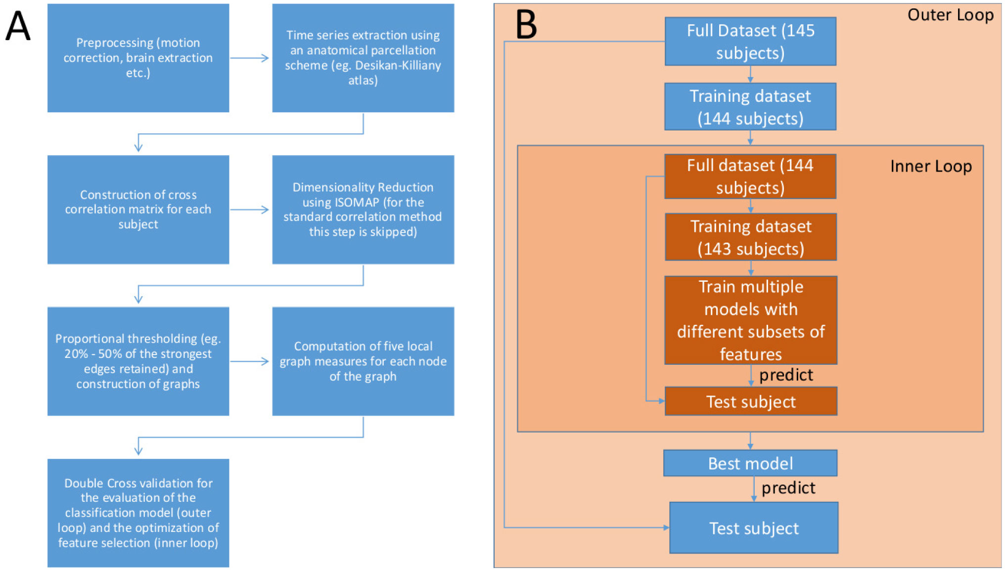
We construct Functional Connectivity Networks (FCN) from resting state fMRI (rsfMRI) recordings towards the classification of brain activity between healthy and schizophrenic subjects using a publicly available dataset (the COBRE dataset) of 145 subjects (74 healthy controls and 71 schizophrenic subjects). First, we match the anatomy of the brain of each individual to the Desikan-Killiany brain atlas. Then, we use the conventional approach of correlating the parcellated time series to construct FCN and ISOMAP, a nonlinear manifold learning algorithm to produce low-dimensional embeddings of the correlation matrices. For the classification analysis, we computed five key local graph-theoretic measures of the FCN and used the LASSO and Random Forest (RF) algorithms for feature selection. For the classification we used standard linear Support Vector Machines. The classification performance is tested by a double cross-validation scheme (consisting of an outer and an inner loop of “Leave one out” cross-validation (LOOCV)). The standard cross-correlation methodology produced a classification rate of 73.1%, while ISOMAP resulted in 79.3%, thus providing a simpler model with a smaller number of features as chosen from LASSO and RF, namely the participation coefficient of the right thalamus and the strength of the right lingual gyrus.
Citation: Ioannis K Gallos, Kostakis Gkiatis, George K Matsopoulos, Constantinos Siettos. ISOMAP and machine learning algorithms for the construction of embedded functional connectivity networks of anatomically separated brain regions from resting state fMRI data of patients with Schizophrenia[J]. AIMS Neuroscience, 2021, 8(2): 295-321. doi: 10.3934/Neuroscience.2021016
We construct Functional Connectivity Networks (FCN) from resting state fMRI (rsfMRI) recordings towards the classification of brain activity between healthy and schizophrenic subjects using a publicly available dataset (the COBRE dataset) of 145 subjects (74 healthy controls and 71 schizophrenic subjects). First, we match the anatomy of the brain of each individual to the Desikan-Killiany brain atlas. Then, we use the conventional approach of correlating the parcellated time series to construct FCN and ISOMAP, a nonlinear manifold learning algorithm to produce low-dimensional embeddings of the correlation matrices. For the classification analysis, we computed five key local graph-theoretic measures of the FCN and used the LASSO and Random Forest (RF) algorithms for feature selection. For the classification we used standard linear Support Vector Machines. The classification performance is tested by a double cross-validation scheme (consisting of an outer and an inner loop of “Leave one out” cross-validation (LOOCV)). The standard cross-correlation methodology produced a classification rate of 73.1%, while ISOMAP resulted in 79.3%, thus providing a simpler model with a smaller number of features as chosen from LASSO and RF, namely the participation coefficient of the right thalamus and the strength of the right lingual gyrus.

| [1] |
Bhugra D (2005) The global prevalence of schizophrenia. PLoS Med 2: e151. doi: 10.1371/journal.pmed.0020151

|
| [2] |
Friston KJ (1998) The disconnection hypothesis. Schizophr Res 30: 115-125. doi: 10.1016/S0920-9964(97)00140-0
|
| [3] |
Liu Y, Liang M, Zhou Y, et al. (2008) Disrupted small-world networks in schizophrenia. Brain 131: 945-961. doi: 10.1093/brain/awn018
|
| [4] |
Lynall ME, Bassett DS, Kerwin R, et al. (2010) Functional connectivity and brain networks in schizophrenia. J Neurosci 30: 9477-9487. doi: 10.1523/JNEUROSCI.0333-10.2010
|
| [5] |
Griffa A, Baumann PS, Ferrari C, et al. (2015) Characterizing the connectome in schizophrenia with diffusion spectrum imaging. Hum Brain Mapp 36: 354-366. doi: 10.1002/hbm.22633
|
| [6] |
Biswal BB (2012) Resting state fMRI: a personal history. Neuroimage 62: 938-944. doi: 10.1016/j.neuroimage.2012.01.090
|
| [7] |
Dong D, Wang Y, Chang X, et al. (2018) Dysfunction of large-scale brain networks in schizophrenia: a meta-analysis of resting-state functional connectivity. Schizophr Bull 44: 168-181. doi: 10.1093/schbul/sbx034
|
| [8] |
Smith SM, Beckmann CF, Andersson J, et al. (2013) Resting-state fMRI in the human connectome project. Neuroimage 80: 144-168. doi: 10.1016/j.neuroimage.2013.05.039
|
| [9] |
Moussa MN, Steen MR, Laurienti PJ, et al. (2012) Consistency of Network Modules in Resting-State fMRI Connectome Data. PloS One 7: e44428. doi: 10.1371/journal.pone.0044428
|
| [10] |
Smith SM, Fox PT, Miller KL, et al. (2009) Correspondence of the brain's functional architecture during activation and rest. Proce Natl Acad Sci 106: 13040-13045. doi: 10.1073/pnas.0905267106
|
| [11] |
Damoiseaux JS, Rombouts SARB, Barkhof F, et al. (2006) Consistent resting-state networks across healthy subjects. Proce Natl Acad Sci 103: 13848-13853. doi: 10.1073/pnas.0601417103
|
| [12] |
Argyelan M, Ikuta T, DeRosse P, et al. (2014) Resting-state fMRI connectivity impairment in schizophrenia and bipolar disorder. Schizophr Bull 40: 100-110. doi: 10.1093/schbul/sbt092
|
| [13] |
Arribas JI, Calhoun VD, Adali T (2010) Automatic Bayesian classification of healthy controls, bipolar disorder, and schizophrenia using intrinsic connectivity maps from FMRI data. IEEE Transa Biomed Eng 57: 2850-2860. doi: 10.1109/TBME.2010.2080679
|
| [14] |
Matsubara T, Tashiro T, Uehara K (2019) Deep neural generative model of functional MRI images for psychiatric disorder diagnosis. IEEE Transa Biomed Eng 66: 2768-2779. doi: 10.1109/TBME.2019.2895663
|
| [15] |
Xiang Y, Wang J, Tan G, et al. (2020) Schizophrenia identification using multi-view graph measures of functional brain networks. Front Bioeng Biotechnol 7: 479. doi: 10.3389/fbioe.2019.00479
|
| [16] | Anderson A, Cohen MS (2013) Decreased small-world functional network connectivity and clustering across resting state networks in schizophrenia: an fMRI classification tutorial. Front Hum Neurosci 7: 520. |
| [17] |
Arbabshirani MR, Kiehl KA, Pearlson DG (2013) Classification of schizophrenia patients based on resting-state functional network connectivity. Front Neurosci 7: 133. doi: 10.3389/fnins.2013.00133
|
| [18] |
Cheng H, Newman S, Goñi J, et al. (2015) Classification of schizophrenia patients based on restingstate functional network connectivity. Schizophr Res 168: 345-352. doi: 10.1016/j.schres.2015.08.011
|
| [19] |
Moghimi P, Lim KO, Netoff TI (2018) Data Driven Classification Using fMRI Network Measures: Application to Schizophrenia. Front Neuroinform 12: 71. doi: 10.3389/fninf.2018.00071
|
| [20] |
Sundermann B, Herr D, Schwindt W, et al. (2014) Multivariate classification of blood oxygen level–dependent fMRI data with diagnostic intention: a clinical perspective. Am J Neuroradiol 35: 848-855. doi: 10.3174/ajnr.A3713
|
| [21] |
Cai XL, Xie DJ, Madsen KH, et al. (2020) Generalizability of machine learning for classification of schizophrenia based on resting-state functional MRI data. Hum Brain Mapp 41: 172-184. doi: 10.1002/hbm.24797
|
| [22] | Du W, Calhoun VD, Li H, et al. (2012) High classification accuracy for schizophrenia with rest and task fMRI data. Front Hum Neurosci 6: 145. |
| [23] |
Pereira F, Mitchell T, Botvinick M (2009) Machine learning classifiers and fMRI: a tutorial overview. Neuroimage 45: S199-S209. doi: 10.1016/j.neuroimage.2008.11.007
|
| [24] |
Krstajic D, Buturovic LJ, Leahy DE, et al. (2014) Cross-validation pitfalls when selecting and assessing regression and classification models. J Cheminform 6: 1-15. doi: 10.1186/1758-2946-6-10
|
| [25] |
Pettersson-Yeo W, Allen P, Benetti S, et al. (2011) Dysconnectivity in schizophrenia: where are we now? Neurosci Biobehav Rev 35: 1110-1124. doi: 10.1016/j.neubiorev.2010.11.004
|
| [26] |
Fekete T, Wilf M, Rubin D, et al. (2013) Combining classification with fMRI-derived complex network measures for potential neurodiagnostics. PloS One 8: e62867. doi: 10.1371/journal.pone.0062867
|
| [27] | Gallos IK, Galaris E, Siettos CIConstruction of embedded fMRI resting-state functional connectivity networks using manifold learning. Cogn Neurodyn (2020) . |
| [28] |
Lombardi A, Guaragnella C, Amoroso N, et al. (2019) Modelling cognitive loads in schizophrenia by means of new functional dynamic indexes. NeuroImage 195: 150-164. doi: 10.1016/j.neuroimage.2019.03.055
|
| [29] |
Hyv¨arinen A, Oja E (2000) Independent component analysis: algorithms and applications. Neural Netw 13: 411-430. doi: 10.1016/S0893-6080(00)00026-5
|
| [30] |
Haak KV, Marquand AF, Beckmann CF (2018) Connectopic mapping with resting-state fMRI. Neuroimage 170: 83-94. doi: 10.1016/j.neuroimage.2017.06.075
|
| [31] |
Desikan RS, Ségonne F, Fischl B, et al. (2006) An automated labeling system for subdividing the human cerebral cortex on MRI scans into gyral based regions of interest. Neuroimage 31: 968-980. doi: 10.1016/j.neuroimage.2006.01.021
|
| [32] |
Kabbara A, Falou WEL, Khalil M, et al. (2017) The dynamic functional core network of the human brain at rest. Sci Rep 7: 1-16. doi: 10.1038/s41598-017-03420-6
|
| [33] |
Tenenbaum JB, De Silva V, Langford JC (2000) A global geometric framework for nonlinear dimensionality reduction. Science 290: 2319-2323. doi: 10.1126/science.290.5500.2319
|
| [34] | Liu J, Li M, Pan Y, et al. (2017) Complex brain network analysis and its applications to brain disorders: a survey. Complexity 2017: 1-27. |
| [35] |
Jenkinson M, Bannister P, Brady M, et al. (2002) Improved optimization for the robust and accurate linear registration and motion correction of brain images. Neuroimage 17: 825-841. doi: 10.1006/nimg.2002.1132
|
| [36] |
Smith SM (2002) Fast robust automated brain extraction. Hum Brain Mapp 17: 143-155. doi: 10.1002/hbm.10062
|
| [37] |
Pruim RHR, Mennes M, van Rooij D, et al. (2015) ICA-AROMA: A robust ICA-based strategy for removing motion artifacts from fMRI data. Neuroimage 112: 267-277. doi: 10.1016/j.neuroimage.2015.02.064
|
| [38] |
Kalcher K, Boubela RN, Huf W, et al. (2014) The spectral diversity of resting-state fluctuations in the human brain. PloS One 9: e93375. doi: 10.1371/journal.pone.0093375
|
| [39] |
Fischl B (2012) FreeSurfer. Neuroimage 62: 774-781. doi: 10.1016/j.neuroimage.2012.01.021
|
| [40] |
Hyde JS, Jesmanowicz A (2012) Cross-correlation: an fMRI signal-processing strategy. Neuroimage 62: 848-851. doi: 10.1016/j.neuroimage.2011.10.064
|
| [41] |
van den Heuvel MP, de Lange SC, Zalesky A, et al. (2017) Proportional thresholding in restingstate fMRI functional connectivity networks and consequences for patient-control connectome studies: Issues and recommendations. Neuroimage 152: 437-449. doi: 10.1016/j.neuroimage.2017.02.005
|
| [42] |
Dimitriadis SI, Antonakakis M, Simos P, et al. (2017) Data-driven topological filtering based on orthogonal minimal spanning trees: application to multigroup magnetoencephalography restingstate connectivity. Brain Connect 7: 661-670. doi: 10.1089/brain.2017.0512
|
| [43] |
Dimitriadis SI, Salis C, Tarnanas I, et al. (2017) Topological filtering of dynamic functional brain networks unfolds informative chronnectomics: a novel data-driven thresholding scheme based on orthogonal minimal spanning trees (OMSTs). Front Neuroinform 11: 28. doi: 10.3389/fninf.2017.00028
|
| [44] | Dijkstra EW (1959) A note on two problems in connexion with graphs. Front Neuroinform 1: 269-271. |
| [45] |
Kruskal JB (1964) Multidimensional scaling by optimizing goodness of fit to a nonmetric hypothesis. Psychometrika 29: 1-27. doi: 10.1007/BF02289565
|
| [46] | Saul LK, Weinberger KQ, Ham JH, et al. (2006) Spectral methods for dimensionality reduction. Semisupervised Learning Cambridge, MA, USA: The MIT Press, 292-308. |
| [47] | Oksanen J, Kindt R, Legendre P, et al. (2007) The vegan package. Community Ecol Package 10: 631-637. |
| [48] | Team, R Core R: A language and environment for statistical computing (2013) . |
| [49] |
Rubinov M, Sporns O (2010) Complex network measures of brain connectivity: uses and interpretations. Neuroimage 52: 1059-1069. doi: 10.1016/j.neuroimage.2009.10.003
|
| [50] |
Blondel VD, Guillaume JL, Lambiotte R, et al. (2008) Fast unfolding of communities in large networks. J Stat Mech Theory Exp 2008: P10008. doi: 10.1088/1742-5468/2008/10/P10008
|
| [51] |
Barrat A, Barthélemy M, Pastor-Satorras R, et al. (2004) The architecture of complex weighted networks. Proc Natl Acad Sci USA 101: 3747-3752. doi: 10.1073/pnas.0400087101
|
| [52] |
Power JD, Schlaggar BL, Lessov-Schlaggar CN, et al. (2013) Evidence for hubs in human functional brain networks. Neuron 79: 798-813. doi: 10.1016/j.neuron.2013.07.035
|
| [53] | Csardi G, Nepusz T (2006) The igraph software package for complex network research. InterJournal Complex Syst 1695: 1-9. |
| [54] |
Chan MK, Krebs MO, Cox D, et al. (2015) Development of a blood-based molecular biomarker test for identification of schizophrenia before disease onset. Transl Psychiatry 5: e601. doi: 10.1038/tp.2015.91
|
| [55] |
Usai MG, Goddard ME, Hayes BJ (2009) LASSO with cross-validation for genomic selection. Genet Res 91: 427-436. doi: 10.1017/S0016672309990334
|
| [56] |
Friedman J, Hastie T, Tibshirani R (2010) Regularization paths for generalized linear models via coordinate descent. J Stat Softw 33: 1-22. doi: 10.18637/jss.v033.i01
|
| [57] | Hastie T, Tibshirani R, Friedman J (2009) The elements of statistical learning: data mining, inference, and prediction New York City, USA: Springer. |
| [58] |
Breiman L (2001) Random forests. Mach Learn 45: 5-32. doi: 10.1023/A:1010933404324
|
| [59] |
Loh WY (2011) Classification and regression trees. WIRES Data Min Knowl 1: 14-23. doi: 10.1002/widm.8
|
| [60] |
Menze BH, Kelm BM, Masuch R, et al. (2009) A comparison of random forest and its Gini importance with standard chemometric methods for the feature selection and classification of spectral data. BMC Bioinformatics 10: 213. doi: 10.1186/1471-2105-10-213
|
| [61] |
Zhu X, Du X, Kerich M, et al. (2018) Random forest based classification of alcohol dependence patients and healthy controls using resting state MRI. Neurosci Lett 676: 27-33. doi: 10.1016/j.neulet.2018.04.007
|
| [62] |
Kesler SR, Rao A, Blayney DW, et al. (2017) Predicting long-term cognitive outcome following breast cancer with pre-treatment resting state fMRI and random forest machine learning. Front Hum Neurosci 11: 555. doi: 10.3389/fnhum.2017.00555
|
| [63] |
Ceriani L, Verme P (2012) The origins of the Gini index: extracts from Variabilità e Mutabilità (1912) by Corrado Gini. J Econ Inequal 10: 421-443. doi: 10.1007/s10888-011-9188-x
|
| [64] |
Strobl C, Boulesteix AL, Augustin T (2007) Unbiased split selection for classification trees based on the Gini index. Comput Stat Data Anal 52: 483-501. doi: 10.1016/j.csda.2006.12.030
|
| [65] | Louppe G, Wehenkel L, Sutera A, et al. (2013) Understanding variable importances in forests of randomized trees. Adv Neural Inf Process Syst 26: 431-439. |
| [66] |
Behnamian A, Millard K, Banks SN, et al. (2017) A systematic approach for variable selection with random forests: achieving stable variable importance values. IEEE Geosci Remote S 14: 1988-1992. doi: 10.1109/LGRS.2017.2745049
|
| [67] | RColorBrewer S, Liaw A, Wiener M, et al. Package ‘randomForest’ (2018) . |
| [68] |
Kuhn M (2008) Building predictive models in R using the caret package. J Stat Softw 28: 1-26. doi: 10.18637/jss.v028.i05
|
| [69] |
Nieuwenhuis M, van Haren NE, Pol HEH, et al. (2012) Classification of schizophrenia patients and healthy controls from structural MRI scans in two large independent samples. Neuroimage 61: 606-612. doi: 10.1016/j.neuroimage.2012.03.079
|
| [70] |
Fan Y, Liu Y, Wu H, et al. (2011) Discriminant analysis of functional connectivity patterns on Grassmann manifold. Neuroimage 56: 2058-2067. doi: 10.1016/j.neuroimage.2011.03.051
|
| [71] |
Salman MS, Du Y, Lin D, et al. (2019) Group ICA for identifying biomarkers in schizophrenia: ‘Adaptive’ networks via spatially constrained ICA show more sensitivity to group differences than spatio-temporal regression. NeuroImage Clin 22: 101747. doi: 10.1016/j.nicl.2019.101747
|
| [72] |
Himberg J, Hyvärinen A, Esposito F (2004) Validating the independent components of neuroimaging time series via clustering and visualization. Neuroimage 22: 1214-1222. doi: 10.1016/j.neuroimage.2004.03.027
|
| [73] | Cole DM, Smith SM, Beckmann CF (2010) Advances and pitfalls in the analysis and interpretation of resting-state FMRI data. Front Syst Neurosci 4: 8. |
| [74] |
Andreasen NC (1997) The role of the thalamus in schizophrenia. Can J Psychiatry 42: 27-33. doi: 10.1177/070674379704200104
|
| [75] |
Byne W, Hazlett EA, Buchsbaum MS, et al. (2009) The thalamus and schizophrenia: current status of research. Acta Neuropathol 117: 347-368. doi: 10.1007/s00401-008-0404-0
|
| [76] |
Pergola G, Selvaggi P, Trizio S, et al. (2015) The role of the thalamus in schizophrenia from a neuroimaging perspective. Neurosci Biobehav Rev 54: 57-75. doi: 10.1016/j.neubiorev.2015.01.013
|
| [77] |
Bogousslavsky J, Miklossy J, Deruaz JP, et al. (1987) Lingual and fusiform gyri in visual processing: a clinico-pathologic study of superior altitudinal hemianopia. J Neurol Neurosurg Psychiatry 50: 607-614. doi: 10.1136/jnnp.50.5.607
|
| [78] |
Mechelli A, Humphreys GW, Mayall K, et al. (2000) Differential effects of word length and visual contrast in the fusiform and lingual gyri during reading. Proc Biol Sci 267: 1909-1913. doi: 10.1098/rspb.2000.1229
|
| [79] |
Yu T, Li Y, Fan F, et al. (2018) Decreased gray matter volume of cuneus and lingual gyrus in schizophrenia patients with tardive dyskinesia is associated with abnormal involuntary movement. Sci Rep 8: 1-7. doi: 10.1038/s41598-017-17765-5
|
| [80] | Kogata T, lidaka T (2018) A review of impaired visual processing and the daily visual world in patients with schizophrenia. Nagoya J Med Sci 80: 317-328. |
| [81] |
Yamamoto M, Bagarinao E, Kushima I, et al. (2020) Support vector machine-based classification of schizophrenia patients and healthy controls using structural magnetic resonance imaging from two independent sites. PloS One 15: e0239615. doi: 10.1371/journal.pone.0239615
|
| [82] |
Tohid H, Faizan M, Faizan U (2015) Alterations of the occipital lobe in schizophrenia. Neurosciences 20: 213-224. doi: 10.17712/nsj.2015.3.20140757
|


Figures(8) / Tables(3)

Ioannis K Gallos, Kostakis Gkiatis, George K Matsopoulos, Constantinos Siettos. ISOMAP and machine learning algorithms for the construction of embedded functional connectivity networks of anatomically separated brain regions from resting state fMRI data of patients with Schizophrenia[J]. AIMS Neuroscience, 2021, 8(2): 295-321. doi: 10.3934/Neuroscience.2021016


 DownLoad: