In this paper we introduce and analyze a non-standard discretized SIS epidemic model for a homogeneous population. The presented model is a discrete version of the continuous model known from literature and used by us for building a model for a heterogeneous population. Firstly, we discuss basic properties of the discrete system. In particular, boundedness of variables and positivity of solutions of the system are investigated. Then we focus on stability of stationary states. Results for the disease-free stationary state are depicted with the use of a basic reproduction number computed for the system. For this state we also manage to prove its global stability for a given condition. It transpires that the behavior of the disease-free state is the same as its behavior in the analogous continuous system. In case of the endemic stationary state, however, the results are presented with respect to a step size of discretization. Local stability of this state is guaranteed for a sufficiently small critical value of the step size. We also conduct numerical simulations confirming theoretical results about boundedness of variables and global stability of the disease-free state of the analyzed system. Furthermore, the simulations ascertain a possibility of appearance of Neimark-Sacker bifurcation for the endemic state. As a bifurcation parameter the step size of discretization is chosen. The simulations suggest the appearance of a supercritical bifurcation.
Citation: Marcin Choiński, Mariusz Bodzioch, Urszula Foryś. A non-standard discretized SIS model of epidemics[J]. Mathematical Biosciences and Engineering, 2022, 19(1): 115-133. doi: 10.3934/mbe.2022006
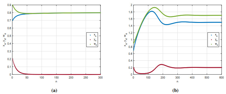
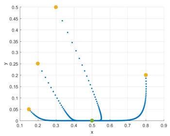
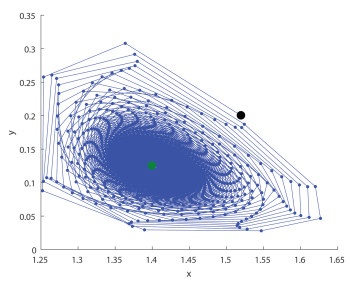
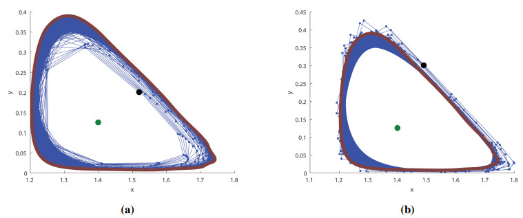
In this paper we introduce and analyze a non-standard discretized SIS epidemic model for a homogeneous population. The presented model is a discrete version of the continuous model known from literature and used by us for building a model for a heterogeneous population. Firstly, we discuss basic properties of the discrete system. In particular, boundedness of variables and positivity of solutions of the system are investigated. Then we focus on stability of stationary states. Results for the disease-free stationary state are depicted with the use of a basic reproduction number computed for the system. For this state we also manage to prove its global stability for a given condition. It transpires that the behavior of the disease-free state is the same as its behavior in the analogous continuous system. In case of the endemic stationary state, however, the results are presented with respect to a step size of discretization. Local stability of this state is guaranteed for a sufficiently small critical value of the step size. We also conduct numerical simulations confirming theoretical results about boundedness of variables and global stability of the disease-free state of the analyzed system. Furthermore, the simulations ascertain a possibility of appearance of Neimark-Sacker bifurcation for the endemic state. As a bifurcation parameter the step size of discretization is chosen. The simulations suggest the appearance of a supercritical bifurcation.

| [1] | J. Liu, B. Peng, T. Zhang, Effect of discretization on dynamical behavior of SEIR and SIR models with nonlinear incidence, Appl. Math. Lett., 39 (2015), 60–66. doi: 10.1016/j.aml.2014.08.012. |
| [2] | S. Side, A. M. Utami, Sukarna, M. I. Pratama, Numerical solution of SIR model for transmission of tuberculosis by Runge–Kutta method, J. Phys. Conf. Ser., 1040 (2018). doi: 10.1088/1742-6596/1040/1/012021. |
| [3] | R. E. Mickens, Nonstandard Finite Difference Models of Differential Equations, World Scientific, Atlanta, 1993. doi: 10.1142/2081. |
| [4] | H. Al-Kahby, F. Dannan, S. Elaydi, Non-standard discretization methods for some biological models, in Applications of Nonstandard Finite Difference Schemes, (2000), 155–180. doi: 10.1142/9789812813251_0004. |
| [5] | Y. A. Kuznetsov, Elements of Applied Bifurcation Theory, 2$^nd$ edition, Springer-Verlag, New York, 1998. doi: 10.1007/b98848. |
| [6] | Z. Enatsu, Z. Teng, C. Jia, C. Zhang, L. Zhang, Dynamical analysis and chaos control of a discrete SIS epidemic model, Adv. Differ. Equations, 58 (2014), 1–20. doi: 10.1186/1687-1847-2014-58. |
| [7] | D. A. Kessler, Epidemic size in the SIS model of endemic infections, J. Appl. Probab., 45 (2008), 757–778. doi: 10.1239/jap/1222441828. |
| [8] | M. Martcheva, An Introduction to Mathematical Epidemiology, Springer, New York, 2015. doi: 10.1007/978-1-4899-7612-3. |
| [9] | R. N. Shalan, R. Shireen, A. H. Lafta, Discrete an SIS model with immigrants and treatment, J. Interdiscip. Math., 24 (2021), 1201–1206. doi: 10.1080/09720502.2020.1814496. |
| [10] | W. L. I. Roeger, Dynamically consisent discrete-time SI and SIS epidemic models, Discrete Contin. Dyn. Syst., 2013 (2013), {653–662}. doi: 10.3934/proc.2013.2013.653. |
| [11] | M. T. Hoang, O. F. Egbelowo, Nonstandard finite difference schemes for solving an SIS epidemic model with standard incidence, Rend. Circolo Mat. Palermo Ser. 2, 69 (2020), 753–769. doi: 10.1007/s12215-019-00436-x. |
| [12] | Y. Enatsu, Y. Nakata, Y. Muroya, Global stability for a discrete SIS epidemic model with immigration of infectives, J. Differ. Equations Appl., 18 (2012), 1913–1924. doi: 10.1080/10236198.2011.602973. |
| [13] | Y. Xie, Z. Wang, J. Lu, Y. Li, Stability analysis and control strategies for a new SIS epidemic model in heterogeneous networks, Appl. Math. Comput., 383 (2020). doi: 10.1016/j.amc.2020.125381. |
| [14] | Y. Xie, Z. Wang, Transmission dynamics, global stability and control strategies of a modified SIS epidemic model on complex networks with an infective medium, Math. Comput. Simul., 188 (2021), 23–34. doi: 10.1016/j.matcom.2021.03.029. |
| [15] | X. Wang, Z. Wang, H. Shen, Dynamical analysis of a discrete-time SIS epidemic model on complex networks, Appl. Math. Lett., 94 (2019), 292–299. doi: 10.1016/j.aml.2019.03.011. |
| [16] | D. B. Saakian, A simple statistical physics model for the epidemic with incubation period, Chin. J. Phys., 73 (2021), 546–551. doi: 10.1016/j.cjph.2021.07.007. |
| [17] | M. Bodzioch, M. Choiński, U. Foryś, SIS criss-cross model of tuberculosis in heterogeneous population, Discrete Contin. Dyn. Syst. Ser. B, 24 (2019), 2169–2188. doi: 10.3934/dcdsb.2019089. |
| [18] | M. Choiński, M. Bodzioch, U. Foryś, Simple criss-cross model of epidemic for heterogeneous populations, Commun. Nonlinear Sci. Numer. Simul., 79 (2019), 1–17. doi: 10.1016/j.cnsns.2019.104920. |
| [19] | M. Choiński, M. Bodzioch, U. Foryś, Simple discrete SIS criss-cross model of tuberculosis in heterogeneous population of homeless and non-homeless people, Math. Appl., 47 (2019), 103–115. doi: 10.14708/ma.v47i1.6496. |
| [20] | L. J. S. Allen, P. van den Driessche, The basic reproduction number in some discrete time epidemic models, J. Differ. Equations Appl., 14 (2008), 1127–1147. doi: 10.1080/10236190802332308. |
Figures(4)

Marcin Choiński, Mariusz Bodzioch, Urszula Foryś. A non-standard discretized SIS model of epidemics[J]. Mathematical Biosciences and Engineering, 2022, 19(1): 115-133. doi: 10.3934/mbe.2022006


 DownLoad: