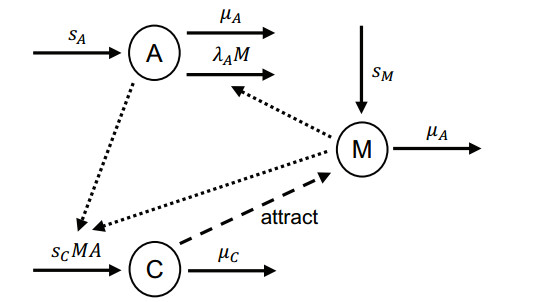
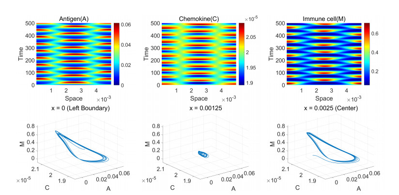
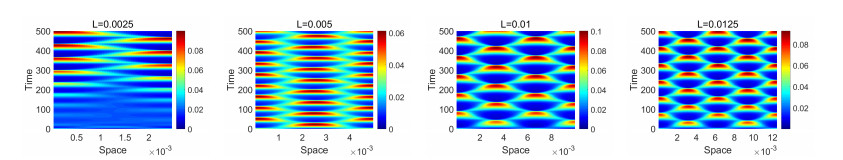
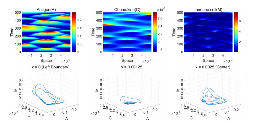
This paper studies a reaction-diffusion-advection system describing a directed movement of immune cells toward chemokines during the immune process. We investigate the global solvability of the model based on the bootstrap argument for minimal chemotaxis models. We also examine the stability of nonconstant steady states and the existence of periodic orbits from theoretical aspects of bifurcation analysis. Through numerical simulations, we observe the occurrence of steady or time-periodic pattern formations.
Citation: Changwook Yoon, Sewoong Kim, Hyung Ju Hwang. Global well-posedness and pattern formations of the immune system induced by chemotaxis[J]. Mathematical Biosciences and Engineering, 2020, 17(4): 3426-3449. doi: 10.3934/mbe.2020194
This paper studies a reaction-diffusion-advection system describing a directed movement of immune cells toward chemokines during the immune process. We investigate the global solvability of the model based on the bootstrap argument for minimal chemotaxis models. We also examine the stability of nonconstant steady states and the existence of periodic orbits from theoretical aspects of bifurcation analysis. Through numerical simulations, we observe the occurrence of steady or time-periodic pattern formations.

| [1] |
P. Devreotes, C. Janetopoulos, Eukaryotic chemotaxis: Distinctions between directional sensing and polarization, J. Biol. Chem., 278 (2003), 20445-20448. doi: 10.1074/jbc.R300010200

|
| [2] |
D. V. Zhelev, A. M. Alteraifi, D. Chodniewicz, Controlled pseudopod extension of human neutrophils stimulated with different chemoattractants, Biophys. J., 87 (2004), 688-695. doi: 10.1529/biophysj.103.036699
|
| [3] | O. Akbari, G. J. Freeman, E. H. Meyer, E. A. Greenfield, T. T. Chang, A. H. Sharpe, et al., Antigen-specific regulatory t cells develop via the icos-icos-ligand pathway and inhibit allergeninduced airway hyperreactivity, Nat. Med., 8 (2002), 1024-1032. |
| [4] | J. E. Gereda, D. Y. M. Leung, A. Thatayatikom, J. E. Streib, M. R. Price, Relation between house-dust endotoxin exposure, type 1 T-cell development, and allergen sensitisation in infants at high risk of asthma, The lancet, 355 (2000), 1680-1683. |
| [5] |
R. Eftimie, J. J. Gillard, D. A. Cantrell, Mathematical models for immunology: Current state of the art and future research directions, Bull. Math. Biol., 78 (2016), 2091-2134. doi: 10.1007/s11538-016-0214-9
|
| [6] |
M. A. Fishman, A. S. Perelson, Modeling T cell-antigen presenting cell interactions, J. Theor. Biol., 160 (1993), 311-342. doi: 10.1006/jtbi.1993.1021
|
| [7] |
F. Groß, M. Fridolin, U. Behn, Mathematical modeling of allergy and specific immunotherapy: Th1-Th2-Treg interactions, J. Theor. Biol., 269 (2011), 70-78. doi: 10.1016/j.jtbi.2010.10.013
|
| [8] | A. B. Pigozzo, G. C. Macedo, R. W. D. Santos, M. Lobosco, On the computational modeling of the innate immune system, BMC Bioinf., 14 (2013), S7. |
| [9] |
B. Su, W. Zhou, K. S. Dorman, D. E. Jones, Mathematical modelling of immune response in tissues, Comput. Math. Methods Med., 10 (2009), 9-38. doi: 10.1080/17486700801982713
|
| [10] |
S. Lee, S. Kim, Y. Oh, H. J. Hwang, Mathematical modeling and its analysis for instability of the immune system induced by chemotaxis, J. Math. Biol., 75 (2017), 1101-1131. doi: 10.1007/s00285-017-1108-7
|
| [11] |
E. F. Keller, L. A. Segel, Initiation of slime mold aggregation viewed as an instability, J. Theor. Biol., 26 (1970), 399-415. doi: 10.1016/0022-5193(70)90092-5
|
| [12] |
H. Gajewski, K. Zachariasand, K. Gröger, Global behaviour of a reaction-diffusion system modelling chemotaxis, Math. Nachr., 195 (1998), 77-114. doi: 10.1002/mana.19981950106
|
| [13] | T. Nagai, Blow-up of radially symmetric solutions to a chemotaxis system, Adv. Math. Sci. Appl., 5 (1995), 581-601. |
| [14] |
T. Nagai, Global existence of solutions to a parabolic system for chemotaxis in two space dimensions, Nonlinear Anal. Theory Method Appl., 30 (1997), 5381-5388. doi: 10.1016/S0362-546X(97)00395-7
|
| [15] | T. Nagai, T. Senba, K. Yoshida, Application of the trudinger-moser inequah. ty to a parabolic system of chemotaxis, Funkc. Ekvacioj, 40 (1997), 411-433. |
| [16] | K. Osaki, A. Yagi, Finite dimensional attractor for one-dimensional Keller-Segel equations, Funkc. Ekvacioj Ser. I., 44 (2001), 441-470. |
| [17] |
M. Winkler, Aggregation vs. global diffusive behavior in the higher-dimensional Keller-Segel model, J. Differ. Equ., 248 (2010), 2889-2905. doi: 10.1016/j.jde.2010.02.008
|
| [18] | F. Rothe, Global solutions of reaction-diffusion systems, Springer, 2006. |
| [19] | H. Amann, Dynamic theory of quasilinear parabolic equations. Ⅱ. Reaction-diffusion systems, Differ. Integral Equ., 3 (1990), 13-75. |
| [20] | J. Liu, Z. A. Wang, Classical solutions and steady states of an attraction-repulsion chemotaxis in one dimension, J. Biol. Dyn., 6 (2012), 31-41. |
| [21] |
L. Wang, C. Mu, S. Zhou, Boundedness in a parabolic-parabolic chemotaxis system with nonlinear diffusion, Z. Angew. Math. Phys., 65 (2014), 1137-1152. doi: 10.1007/s00033-013-0375-4
|
| [22] | A. Friedman, Partial differential equations of parabolic type, Courier Dover Publications, 2008. |
| [23] |
N. D. Alikakos, Lp bounds of solutions of reaction-diffusion equations, Commun. Partial. Differ. Equ., 4 (1979), 827-868. doi: 10.1080/03605307908820113
|
| [24] |
N. Bellomo, A. Bellouquid, Y. Tao, M. Winkler, Toward a mathematical theory of Keller-Segel models of pattern formation in biological tissues, Math. Models Methods Appl. Sci., 25 (2015), 1663-1763. doi: 10.1142/S021820251550044X
|
| [25] |
T. Ma, S. Wang, Phase transitions for the Brusselator model, J. Math. Phys., 52 (2011), 033501. doi: 10.1063/1.3559120
|
| [26] | T. Ma, S. Wang, Phase transition dynamics, Springer, 2016. |
| [27] |
M. G. Crandall, P. H. Rabinowitz, The Hopf bifurcation theorem in infinite dimensions, Arch. Ration. Mech. Anal., 67 (1977), 53-72. doi: 10.1007/BF00280827
|
| [28] | Q. Wang, J. Yang, L. Zhang, Time periodic and stable patterns of a two-competing-species Keller-Segel chemotaxis model effect of cellular growth, preprint, arXiv preprint arXiv (2015), 1505.06463. |
| [29] |
A. Chertock, A. Kurganov, X. Wang, Y. Wu, On a chemotaxis model with saturated chemotactic flux, Kinet. Relat. Models, 5 (2012), 51-95. doi: 10.3934/krm.2012.5.51
|
| [30] | A. Kurganov, M. Lukacova-Medvidova, Numerical study of two-species chemotaxis models, Discrete Contin. Dyn. Syst. Ser. B, 19 (2014), 131-152. |
| [31] | Y. Kim, S. Lee, Y. S. Kim, S. Lawler, Y. S. Gho, Y. K. Kim, et al., Regulation of Th1/Th2 cells in asthma development: A mathematical model, Math. Biosci. Eng., 10 (2013), 1095-1133. |
| [32] |
T. E. Van Dyke, A. A. Reilly, R. J. Genco, Regression line analysis of neutrophil chemotaxis, Immunopharmacology, 4 (1982), 23-39. doi: 10.1016/0162-3109(82)90023-6
|
Figures(7) / Tables(3)

Changwook Yoon, Sewoong Kim, Hyung Ju Hwang. Global well-posedness and pattern formations of the immune system induced by chemotaxis[J]. Mathematical Biosciences and Engineering, 2020, 17(4): 3426-3449. doi: 10.3934/mbe.2020194


 DownLoad: