Loading [MathJax]/jax/output/SVG/jax.js
Research article Special Issues

Biochemical and biophysical mechanisms underlying the heart and the brain dialog

  • Received: 20 August 2020 Accepted: 18 October 2020 Published: 28 October 2020
  • In this paper, within the so called “neuro-visceral integration model”, it is reviewed the ability of the heart to secrete numerous endocrine mediators, neurotransmitters and substances that regulate the immune function with repercussions on the central nervous system. The heart would also seem to be able to process various information independently, influencing the brain work through the “intrinsic cardiac nervous system” and baroreceptor pathways. In reviewing this matter, further physical mechanisms are also described, including mechanical contractions and deformations, that are involved in the “heart-brain symphony” based on intra-cardiac formation and propagation of blood vortices coupled to electrical signals. The relevance of the role of vorticity of the blood flow in the molecular dynamics and physiological activity is stressed. By resorting to some conceptual and formal aspects of the dissipative quantum model of brain, mechanisms such as the spontaneous breakdown of symmetry in many-body physics, the dynamical formation of long range correlations and their associated Nambu-Goldstone quanta, coherent states and fractal self-similarity are discussed with reference to the heart-brain dialog. Our discussion supports the view that the heart role is more than the one of a muscle responsible of the blood flow. Further related topics such as the formation of aneurysms and vein varices which in our modeling seem to be related to the weakening or loss of vorticity of the blood flow, the role of the recently discovered fluid-filled interstitial structure and the complex network of thick collagen bundles are finally briefly mentioned in the concluding remarks.

    Citation: C. Dal Lin, M. Falanga, E. De Lauro, S. De Martino, G. Vitiello. Biochemical and biophysical mechanisms underlying the heart and the brain dialog[J]. AIMS Biophysics, 2021, 8(1): 1-33. doi: 10.3934/biophy.2021001

    Related Papers:

    [1] Bing Long, Zaifu Jiang . Estimation and prediction for two-parameter Pareto distribution based on progressively double Type-II hybrid censored data. AIMS Mathematics, 2023, 8(7): 15332-15351. doi: 10.3934/math.2023784
    [2] Ahmed Elshahhat, Refah Alotaibi, Mazen Nassar . Statistical inference of the Birnbaum-Saunders model using adaptive progressively hybrid censored data and its applications. AIMS Mathematics, 2024, 9(5): 11092-11121. doi: 10.3934/math.2024544
    [3] Samah M. Ahmed, Abdelfattah Mustafa . Estimation of the coefficients of variation for inverse power Lomax distribution. AIMS Mathematics, 2024, 9(12): 33423-33441. doi: 10.3934/math.20241595
    [4] Magdy Nagy, Khalaf S. Sultan, Mahmoud H. Abu-Moussa . Analysis of the generalized progressive hybrid censoring from Burr Type-Ⅻ lifetime model. AIMS Mathematics, 2021, 6(9): 9675-9704. doi: 10.3934/math.2021564
    [5] Ahmed R. El-Saeed, Ahmed T. Ramadan, Najwan Alsadat, Hanan Alohali, Ahlam H. Tolba . Analysis of progressive Type-Ⅱ censoring schemes for generalized power unit half-logistic geometric distribution. AIMS Mathematics, 2023, 8(12): 30846-30874. doi: 10.3934/math.20231577
    [6] Xue Hu, Haiping Ren . Statistical inference of the stress-strength reliability for inverse Weibull distribution under an adaptive progressive type-Ⅱ censored sample. AIMS Mathematics, 2023, 8(12): 28465-28487. doi: 10.3934/math.20231457
    [7] Heba S. Mohammed . Empirical E-Bayesian estimation for the parameter of Poisson distribution. AIMS Mathematics, 2021, 6(8): 8205-8220. doi: 10.3934/math.2021475
    [8] Amal S. Hassan, Najwan Alsadat, Oluwafemi Samson Balogun, Baria A. Helmy . Bayesian and non-Bayesian estimation of some entropy measures for a Weibull distribution. AIMS Mathematics, 2024, 9(11): 32646-32673. doi: 10.3934/math.20241563
    [9] Mazen Nassar, Refah Alotaibi, Ahmed Elshahhat . Reliability analysis at usual operating settings for Weibull Constant-stress model with improved adaptive Type-Ⅱ progressively censored samples. AIMS Mathematics, 2024, 9(7): 16931-16965. doi: 10.3934/math.2024823
    [10] Refah Alotaibi, Mazen Nassar, Zareen A. Khan, Ahmed Elshahhat . Statistical analysis of stress–strength in a newly inverted Chen model from adaptive progressive type-Ⅱ censoring and modelling on light-emitting diodes and pump motors. AIMS Mathematics, 2024, 9(12): 34311-34355. doi: 10.3934/math.20241635
  • In this paper, within the so called “neuro-visceral integration model”, it is reviewed the ability of the heart to secrete numerous endocrine mediators, neurotransmitters and substances that regulate the immune function with repercussions on the central nervous system. The heart would also seem to be able to process various information independently, influencing the brain work through the “intrinsic cardiac nervous system” and baroreceptor pathways. In reviewing this matter, further physical mechanisms are also described, including mechanical contractions and deformations, that are involved in the “heart-brain symphony” based on intra-cardiac formation and propagation of blood vortices coupled to electrical signals. The relevance of the role of vorticity of the blood flow in the molecular dynamics and physiological activity is stressed. By resorting to some conceptual and formal aspects of the dissipative quantum model of brain, mechanisms such as the spontaneous breakdown of symmetry in many-body physics, the dynamical formation of long range correlations and their associated Nambu-Goldstone quanta, coherent states and fractal self-similarity are discussed with reference to the heart-brain dialog. Our discussion supports the view that the heart role is more than the one of a muscle responsible of the blood flow. Further related topics such as the formation of aneurysms and vein varices which in our modeling seem to be related to the weakening or loss of vorticity of the blood flow, the role of the recently discovered fluid-filled interstitial structure and the complex network of thick collagen bundles are finally briefly mentioned in the concluding remarks.


    In the reliability and life testing experiments, censored samples are common way to save time and reduce the number of failed experimental items. Type-Ⅰ and Type-Ⅱ censoring schemes are the most common censoring schemes used in the life-testing and reliability studies. The mixture of these two schemes is called the hybrid censoring scheme. For more details about the hybrid censoring schemes, see Balakrishnan and Kundu [1]. The main disadvantage of the conventional Type-Ⅰ and Type-Ⅱ and the hybrid censoring schemes is that they do not allow the experimenter to remove the experimental items at any time point other than the terminal point. For this reason, one may use a general censoring scheme which called progressive Type-Ⅱ censoring. In this censoring scheme n items are placed on a test and the number of items to be failed, denoted by m, and the number of items that are removed at each failure time, denoted Ri, are determined in advance. At the time of the first failure x1:m:n, R1 items are randomly removed from the remaining n1 surviving items. Similarly, at the time of the second failure x2:m:n, R2 items of the remaining n2R1 items are randomly removed and so on. At the time xm:m:n, all the remaining nmR1R2Rm1 items are removed. For more information see Balakrishnan and Aggarwala [2] and Balakrishnan [3].

    Kundu and Joarder [4] introduced the Type-Ⅰ progressive hybrid censoring scheme by combining the concepts of progressive and hybrid censoring schemes. In this scheme, n items are placed on a test with the progressive censoring scheme R1,R2,,Rm and the experiment is terminated at T=min(xm:m:n,T), where T is a predetermined time. The drawback of this scheme is that the statistical inference methods will have low efficiency or may not be applicable. Since the number of failures is random and it can be zero or a very small number. To overcome this disadvantage and increase the efficiency of the statistical inference, Ng et al. [5] proposed an adaptive Type-Ⅱ progressive hybrid censoring scheme (A-II PHCS). In the A-II PHCS, the number of failures m and the progressive censoring scheme R1,R2,,Rm are predetermined and the experimental time is allowed to run over the predetermined time T with the flexibility of changing some values of Ri during the experiment. When Xm:m:m<T, then the experiment stops at this time and we will have the conventional progressive Type-Ⅱ censoring scheme. On the other hand, if XJ:m:n<T<XJ+1:m:n, where XJ:m:n is the Jth failure time occur before the predetermined time T and J+1<m, then we adjust the progressive censoring scheme by resetting RJ+1,RJ+2,,Rm1=0 and Rm=nmJi=1Ri. This adaption assures us to terminate the experiment when m is occurred, and guarantee that the total test time will not be too long away from the time T.

    Recently, many authors have studied different distributions based on A-II PHCS. For example, Lin et al. [6], discussed the estimation problem of Weibull distribution. Hemmati et al. [7], discussed the maximum likelihood and approximate maximum likelihood estimation for the log-normal distribution. Mahmoud et al. [8], studied the Bayes estimation of Pareto distribution. Ismail [9], investigated the estimation of Weibull distribution and the acceleration factor under step-stress partially accelerated life test model. AL Sobhi and Soliman [10], studied the estimation of parameters, reliability and hazard functions of the exponentiated Weibull distribution. Nassar and Abu-Kasem [11] and Nassar et al. [12] investigated the estimation problems of inverse Weibull and Weibull distributions, respectively.

    Burr [13] introduced the Burr type-XII distribution as a member of a 12 types of cumulative distribution functions. The Burr type-XII distribution has many applications in various fields including probability theory, reliability, failure time modeling and household income. A random variable X is said to have two-parameters Burr type-XII distribution, denoted by Burr(a,b), if its probability density and reliability functions are given, respectively, by

    f(x)=abxa1(1+xa)(b+1),x>0,a,b>0, (1.1)

    and

    R(x)=(1+xa)b,x>0, (1.2)

    where a and b are shape parameters. The Lomax distribution can be obtained as a special case from Burr(a,b) distribution by stting a=1. Also, when b=1, the Burr(a,b) distribution reduces to the Champernowne distribution. Evans and Ragab [14] discussed the Bayesian inferences from Burr type-XII distribution based on Type-Ⅱ censored scheme. Moore and Papadopoulos [15] used the Bayesian estimation method to estimate the Burr type-XII distribution parameters using three different loss functions. Mousa and Jaheen [16] obtained the Bayesian estimators of the Burr type-XII distribution parameters under progressive Type-Ⅱ censored scheme. Jaheen and Okasha [17] discussed the estimation problem of the Burr type-XII distribution using Bayesian and E-Bayesian estimation using Type-Ⅱ censored scheme. Hanieh and Abdolreza [18] presented the statistical inference and prediction of the Burr type-XII distribution under unified hybrid scheme. See also, Montaser [19], Jia et al. [20] and Arabi and Noori [21].

    To the best of our knowledge, the E-Bayesian estimation of the Burr(a,b) distribution under A-II PHCS has not yet been studied. The main aim of this paper is to investigate the E-Bayesian estimation of the parameter b and the reliability function of the Burr(a,b) distribution under A-II PHCS with the assumption that the parameter a is known. The maximum likelihood method, Bayesian and E-Bayesian estimations are considered using three different prior distributions. The Bayesian and E-Bayesian estimations are discussed based on squared error (SE) and LINEX loss functions. The E-Bayesian properties are studied and the E-Posterior risk is also obtained. A simulation study is conducted to compare the performance of the different estimators of the parameter b and the reliability function. Application to a real data shows that the E-Bayesian estimators perform better than the maximum likelihood and Bayesian estimators.

    The rest of this paper is organized as follows: In Section (2), we obtain the maximum likelihood and Bayesian estimations of the parameter b and the reliability function of Burr(a,b). The E-Bayesian estimation is considered in Section (3). In Section (4), we study the properties of the E-Bayesian estimation. The E-posterior risk of the E-Bayesian estimation is obtained in Section (5). A simulation study is performed in Section (6). A real data is analyzed in Section (7). Finally, the paper is concluded in Section (8).

    Based on adaptive Type-Ⅱ progressive hybrid censoring sample of size m obtained from a life test experiment of n items from the Burr(a,b) distribution, we can write the likelihood function as follows

    L(a,bx_)ambmψ(a;x_)ebP, (2.1)

    where

    x_=(x1,x2,,xm),ψ(a;x_)=mi=1(xa1i1+xai),
    PP(a;x_)=mi=1ln(1+xai)+Ji=1Riln(1+xai)+Rln(1+xam),

    where R=nmJi=1Ri, and xi=xi:m:n for simplicity of notation. Assuming that the parameter a is known, then the maximum likelihood estimate (MLE) of the parameter b is obtained as follows

    ˆbML=mP. (2.2)

    From (2.2) and the invariance property of the maximum likelihood, we can obtain the MLE of the reliability function R(x) by replacing b by its MLE in (1.2).

    In the Bayesian estimation, we assume that the parameter a is known and the parameter b follows the gamma conjugate prior distribution as proposed by Papadopoulos [15] in the following form

    g(b)=θαΓ(α)bα1ebθ,b>0, (2.3)

    where α>0 and θ>0. From (2.1) and (2.3), the posterior density of b given x_ can be written as

    q(bx_)=Abm+α1e(θ+P)b,b>0, (2.4)

    where

    A=(θ+P)m+αΓ(m+α). (2.5)

    To obtain the Bayes estimate of b, we consider two types of loss functions. The first loss function is the SE loss function and the Bayes estimate in this case is the posterior mean. The second one is the LINEX loss function with the Bayes estimate obtained as

    ˆbBL=1zlnE(ezb),z0. (2.6)

    Based on the SE loss function, we can obtain the Bayes estimate of b as follows

    ˆbBS(α,θ)=m+αθ+P, (2.7)

    while the Bayes estimate of b using the LINEX loss function can be obtained from (2.4) and (2.6) by

    ˆbBL(α,θ)=m+αzln(1+zθ+P). (2.8)

    Under the SE loss function, the Bayes estimate of the reliability function can be obtained from (1.2) and (2.4) as

    ˆRBS(x)=(θ+Pθ+P+P)m+α, (2.9)

    where

    P=ln(1+xα).

    Similarly, from (1.2), (2.4) and (2.6), the Bayes estimate of the reliability function under LINEX loss function can be obtained as follows

    ˆRBL(x)=1z[lnE(ezR(t))]=1zln[(θ+P)m+αΓ(m+α)0ezeθPbm+α1e(θ+P)bdb]=1zln[i=0(z)iΓ(i)(θ+Pθ+P+iP)m+α]. (2.10)

    Han [22] introduced the E-Bayesian (Expected Bayesian) estimation to obtain the estimate of the scale parameter of the exponential distribution based on SE loss function. He also derived the properties of the E-Bayesian estimation. For more relevant research about the E-Bayesian estimation, see Han [22,23], Okasha and Wang [24], Azimi et al. [25], Okasha [26,27,28], and Abdallah and Junping [29]. Han [22] stated that the prior distribution of α and θ should be determined to ensure that the prior distribution g(b) is a decreasing function in b. To make sure this condition is satisfied, we obtain the first derivative of g(b) with respect to b as

    dg(b)db=θαΓ(α)bα2ebθ[(α1)bθ],

    where α,θ,b>0. It is noted that when 0<α<1 and θ>0 the function dg(b)b<0, and therefore g(b) is a decreasing function of b. Suppose that α and θ are independent and have the bivariate density function

    π(α,θ)=π1(α)π2(θ),

    then, according to Han [30] the E-Bayesian estimate of the parameter b (expectation of the Bayesian estimate of b) can be obtained as follows

    ˆbEB=DˆbBS(α,θ)π(α,θ)dαdθ, (3.1)

    where ˆbEB(α,θ) is the Bayes estimate of b under any loss function. For more details about E-Bayesian estimation, see Han [22], Jaheen and Okasha [17] and Okasha [26,27,28].

    Here, we obtain the E-Bayesian estimates of the parameter b by considering three different prior distributions of the hyper-parameters α and θ. These prior distributions are selected to show the effect of the different prior distributions on the E-Bayesian estimation of the parameter b. The selected priors distributions are given by

    π1(α,θ)=1cB(u,v)αu1(1α)v1,0<α<1,0<θ<cπ2(α,θ)=2c2B(u,v)(cθ)αu1(1α)v1,0<α<1,0<θ<cπ3(α,θ)=2θc2B(u,v)αu1(1α)v1,0<α<1,0<θ<c}, (3.2)

    where B(u,v) is the beta function. These prior distributions are used by Zeinhum and Okasha [17] to guarantee that g(b) is a decreasing function in b. Now, the E-Bayesian estimates of the parameter b under SE loss function can be obtained from (2.7), (3.1) and (3.2). Using the prior distribution π1(α,θ), the E-Bayesian estimate of b under SE loss function is given by

    ˆbEBS1=DˆbBS(α,θ)π1(α,θ)dθdα=1cB(u,v)10c0(m+αθ+P)αu1(1α)v1dθdα=1c(m+uu+v)ln(1+cP). (3.3)

    Using the same approach, the E-Bayesian estimates of b based on π2(α,θ) and π3(α,θ) are given, respectively, by

    ˆbEBS2=2c(m+uu+v)[(1+Pc)ln(1+cP)1], (3.4)

    and

    ˆbEBS3=2c(m+uu+v)[1Pcln(1+cP)]. (3.5)

    The E-Bayesian estimation of b under LINEX loss function can be obtained by using the different prior distributions of the hyperparameters given in (3.2). For the prior distribution π1(α,θ) and based on (2.8) and (3.1), the E-Bayesian estimate of b is obtained as

    ˆbEBL1=DˆbBL(α,θ)π1(α,θ)dθdα=1czB(u,v)10c0(m+α)αu1(1α)v1ln(1+zθ+P)dθdα=1cz(m+uu+v)[cln(1+zc+P)+(P+z)ln(1+cP+z)Pln(1+cP)]. (3.6)

    Similarly, the E-Bayesian estimates of b using π2(α,θ) and π3(α,θ) are given, respectively, by

    ˆbEBL2=(m+uu+v)[1zln(1+zP)(P+c)2c2zln(1+cP)+(P+z+c)2c2z×ln(1+cP+z)1c] (3.7)

    and

    ˆbEBL3=(m+uu+v)[1zln(1+zc+P)+P2c2zln(1+cP)(P+z)2c2zln(1+cP+z)+1c]. (3.8)

    Based on the SE loss function, the E-Bayesian estimates of the reliability function can be derived by using the three different prior distributions of the hyper-parameters given by (3.2). For the first prior distribution π1(α,θ), the E-Bayesian estimate of the reliability function is obtained from (2.9) and (3.1) as

    ˆREBS1=DˆRBS(t)π1(α,θ)dθdα=1cB(u,v)10c0(θ+Pθ+P+P)m+ααu1(1α)v1dθdα.=1cB(u,v)c0(1+Pθ+P)m(10eαln(θ+Pθ+P+P)αu1(1α)v1dα)dθ.=1cc0(1+Pθ+P)mF1:1(u,u+v;ln(θ+Pθ+P+P))dθ, (3.9)

    where F1:1(.,.;.) is the generalized hypergeometric function. See for more details Gradshteyn and Ryzhik [31]. Similarly, the E-Bayesian estimates of the reliability function based on the prior distributions 2 and 3 are given, respectively, by

    ˆREBS2=2c2c0(cθ)(1+Pθ+P)mF1:1(u,u+v;ln(θ+Pθ+P+P))dθ, (3.10)

    and

    ˆREBS3=2c2c0θ(1+Pθ+P)mF1:1(u,u+v;ln(θ+Pθ+P+P))dθ, (3.11)

    The integrals in (3.9), (3.10) and (3.11) can not be computed in a simple closed forms. Therefore, a numerical techniques should be used to obtain the E-Bayesian estimates of the reliability functions based on the SE loss function using the different prior distributions.

    Under LINEX loss function, the E-Bayesian estimates of the reliability function using the prior distribution πi(α,θ),i=1,2,3, can be obtained from (2.10) and (3.1) as

    ˆREBLi=DˆRBL(t)πi(α,θ)dθdα. (3.12)

    The integrals in (3.12) are very complicated to obtain, so a numerical computations are used to obtain the E-Bayesian estimates of the reliability function under LINEX loss function.

    In this section, we investigate the relations among the different E-Bayesian estimates of the parameter b and the reliability function based on the SE loss function in terms of biases Bi(bEBSi) and Bi(REBSi), i=1,2,3. Moreover, we discuss the relations between the different E-Bayesian estimates of b and the reliability function under the LINEX loss function through the relations between biases, Bi(bEBli) and Bi(REBLi).

    The relations between Bi(bEBSi), Bi(bEBli), Bi(REBSi) and Bi(REBli), i=1,2,3 are described in the following theorems:

    Theorem 1. Let y=cP, c>0, 0<cP<1, and bEBSi are given by (3.3), (3.4) and (3.5).Then we have the following conclusions:

    (i) Bi(bEBS2)<Bi(bEBS1)<Bi(bEBS3),

    (ii) limy0Bi(bEBS1)=limy0Bi(bEBS2)=limy0Bi(bEBS3).

    Proof. (i) From (3.3), (3.4) and (3.5), we have

    Bi(bEBS1)Bi(bEBS2)=Bi(bEBS3)Bi(bEBS1)=1c(m+uu+v)[c+2Pcln(1+cP)2] (4.1)

    For 1<x<1, we have: ln(1+x)=xx22+x33x44+=k=1(1)k1xkk. Let y=cP, when c>0, 0<cP<1, we have:

    [(1+2y1)ln(1+y)2]=(1+2y1)(yy22+y33y44+y55)2=(yy22+y33y44+y55)+(2y+2y232y34+2y45)2=(y26y36)+(3y462y515)+=y26(1y)+y460(98y)+. (4.2)

    From (4.1) and (4.2), we have

    Bi(bEBS1)Bi(bEBS2)=Bi(bEBS3)Bi(bEBS1)>0,

    that is

    Bi(bEBS2)<Bi(bEBS1)<Bi(bEBS3).

    (ii) From (4.1) and (4.2), we get

    limy0(Bi(bEBS1)Bi(bEBS2))=limy0(Bi(bEBS3)Bi(bEBS1))=1c(m+uu+v)limy0{y26(1y)+y460(98y)+}=0.

    That is, limy0Bi(bEBS1)=limy0Bi(bEBS2)=limy0Bi(bEBS3).

    Theorem 2. Let c>0, 0<cP<1, and bEBLi are given by (3.6), (3.7) and (3.8).Then we have the following conclusions:

    (i) Bi(bEBL2)<Bi(bEBL1)<Bi(bEBL3),

    (ii) limPBi(bEBL1)=limPBi(bEBL2)=limPBi(bEBL3),

    Proof. (i) From (3.6), (3.7) and (3.8), we have

    Bi(bEBL1)Bi(bEBL2)=Bi(bEBL3)Bi(bEBL1)=1c2z(m+uu+v)[(P+z)(P+z+c)ln(1+cP+z)P(P+c)ln(1+cP)cz]. (4.3)

    Since,

    [(P+z)(P+z+c)ln(1+cP+z)P(P+c)ln(1+cP)cz]=z+(P+c2c26P+c312P2c420P3+)[P+z+c2c2(P+z)(12(1+cP+z)[13c4(P+z)+c25(P+z)])]=c2P+z(12(1+cP+z)(13c4(P+z)+c25(P+z)))(c26Pc312P2+c420P3). (4.4)

    From (4.3) and (4.4), when c>0, 0<cP<1, we have:

    Bi(bEBL1)Bi(bEBL2)=Bi(bEBL3)Bi(bEBL1)>0,

    that is

    Bi(bEBL2)<Bi(bEBL1)<Bi(bEBL3).

    (ii) From (4.3) and (4.4) we get

    limP(Bi(bEBL1)Bi(bEBL2))=limP(Bi(bEBL3)Bi(bEBL1))=1cz(m+uu+v)(limPc2P+s(12(1+cP+z)(13c4(P+z)+c25(P+z))))1cz(m+uu+v)limP(c26Pc312P2+c420P3).=0. (4.5)

    That is, limPBi(bEBL1)=limPBi(bEBL2)=limPBi(bEBL3).

    Theorem 3. Let c>0, 0<cP<1, and REBSi are given by (3.9), (3.10) and (3.11).Then we have the following conclusions:

    (i) Bi(REBS2)<Bi(REBS1)<Bi(REBS3),

    (ii) limPBi(REBS1)=limPBi(REBS2)=limPBi(REBS3)

    Proof. (i) From (3.9), (3.10) and (3.11), we have

    g(c)=Bi(REBS1)Bi(REBS2)=Bi(REBS3)Bi(REBS1)=10c0(2θc)(θ+Pθ+P+P)m+ααu1(1α)v1c2B(u,v)dθdα (4.6)

    For α(0,1), θ(0,c), (2θc)(θ+Pθ+P+P)m+α and αu1(1α)v1c2B(u,v) are continuous functions and αu1(1α)v1c2B(u,v)>0, by the generalized mean value theorem for definite integrals, there is at least one number α0(0,1) and θ0(0,c) such that

    g(c)=(2θ0c)(θ0+Pθ0+P+P)m+α010c0αu1(1α)v1c2B(u,v)dθdα=2θ0cc(θ0+Pθ0+P+P)m+α0>0. (4.7)

    Therefore, we obtain that

    Bi(REBS1)Bi(REBS2)=Bi(REBS3)Bi(REBS1)>0,

    that is

    Bi(REBS2)<Bi(REBS1)<Bi(REBS3).

    (ii) From (4.6) we get

    limP(Bi(REBS1)Bi(REBS2))=limP(Bi(REBS3)Bi(REBS1))=1c2B(u,v)limP10c0(2θc)(θ+Pθ+P+P)m+ααu1(1α)v1dθdα=1c2B(u,v)10c0(2θc)(limP(θ+Pθ+P+P)m+α)αu1(1α)v1dθdα=0. (4.8)

    That is, limPBi(REBS1)=limPBi(REBS2)=limPBi(REBS3).

    Theorem 4. Let c>0, 0<cP<1, and REBLi are given by (3.12). Then we have the following conclusions:

    (i) Bi(REBL3)<Bi(REBL2)<Bi(REBL1).

    (ii) limPBi(REBL1)=limPBi(REBL2)=limPBi(REBL3)

    Proof. (i) From (3.2) and (3.12), we have

    f(c)=Bi(REBL2)Bi(REBL3)=Bi(REBL1)Bi(REBL2)=10c0Bi(RBL(t))(π1(α,θ)π2(α,θ))dθdα=10c0Bi(RBL(t))(π3(α,θ)π1(α,θ))dθdα=1c2B(u,v)10c0(2θc)ln(i=0(δ)iΓ(i)(θ+Pθ+P+iP)m+α)αu1(1α)v1dθdα. (4.9)

    For α(0,1), θ(0,c), (2θc)ln(i=0(δ)iΓ(i)(θ+Pθ+P+iP)m+α) and αu1(1α)v1c2B(u,v) are continuous functions and αu1(1α)v1c2B(u,v)>0, by the generalized mean value theorem for definite integrals, there is at least one number α1(0,1) and θ1(0,c) such that

    f(c)=(2θ1c)ln(i=0(δ)iΓ(i)(θ1+Pθ1+P+iP)m+α1)10c0αu1(1α)v1c2B(u,v)dθdα=2θ1ccln(i=0(δ)iΓ(i)(θ1+Pθ1+P+iP)m+α1)>0. (4.10)

    Therefore, we obtain that

    Bi(REBL2)Bi(REBL3)=Bi(REBL1)Bi(REBL2)>0,

    that is

    Bi(REBL3)<Bi(REBL2)<Bi(REBL1).

    (ii) From (4.9) we get

    limP(Bi(REBL2)Bi(REBL3))=limP(Bi(REBL1)Bi(REBL2))=10c0limPBi(RBL(t))(π1(α,θ)π2(α,θ))dθdα=10c0limPBi(RBL(t))(π3(α,θ)π1(α,θ))dθdα=1c2B(u,v)limP10c0(2θc)ln[i=0(δ)iΓ(i)(θ+Pθ+P+iP)m+α]αu1(1α)v1dθdα=1c2B(u,v)10c0(2θc)(limPln(i=0(δ)iΓ(i)(θ+Pθ+P+iP)m+α))αu1(1α)v1dθdα=0. (4.11)

    That is, limPBi(REBL1)=limPBi(REBL2)=limPBi(REBL3).

    In this section, we derive the E-posterior risk of the E-Bayesian estimations of the parameter b using the three different prior distributions in (3.2) under SE and LINEX loss functions.

    Let (ˆμ,μ) be any loss function where ˆμ is the Bayes estimator of μ, and q(μ|x_) is the posterior distribution of μ, then the posterior risk (PR) for the Bayesian estimation is

    PR=(ˆμ,μ)q(μ|x_)dμ. (5.1)

    Under SE loss function the PR of the Bayes estimation is the posterior variance. From the posterior distribution in (2.4) we can obtain the PR of Bayesian estimation of b as follows

    PRBS=A0bm+α+1e(θ+P)bdb(m+αθ+P)2=m+α(θ+P)2. (5.2)

    According to Han [23] the E-posterior risk of the E-Bayesian estimation can be obtained as

    PREBS=DPRBSπ(α,θ)dθdα, (5.3)

    where PRBS is the posterior risk defined in (5.2) and π(α,θ) is the prior distribution. Now, from (3.2), (5.2) and (5.3) we can obtain the E-posterior risk of the E-Bayesian estimation under SE loss function as follow

    (i) The E-posterior risk of the E-Bayesian estimation of ˆbEBS1 is

    PREBS1=1cB(u,v)10c0m+α(θ+P)2αu1(1α)v1dθdα=1c2(m+uu+v)(cPcP+c).

    (ii) The E-posterior risk of the E-Bayesian estimation of ˆbEBS2 is

    PREBS2=2c2B(u,v)10c0m+α(θ+P)2(cθ)αu1(1α)v1dθdα=2c2(m+uu+v)(1+ln(P)+cPcP+cPP+cln(T+c)).

    (iii) The E-posterior risk of the E-Bayesian estimation of ˆbEBS3 is

    PREBS3=2c2B(u,v)10c0m+α(θ+P)2θαu1(1α)v1dθdα=2c2(m+uu+v)(ln(P+c)+PP+cln(P)1).

    Using the same approach in the previous subsection we can obtain the posterior risk of the Bayes estimate of b under LINEX loss function as follows

    PRBL=0(ez(ˆbBLb)z(ˆbBLb)1)bm+α1e(θ+T)bdb=(ezˆbBLE(ezb)zˆbBL+zE(b)1)=(ezˆbBLezˆbBLzˆbBL+zˆbBS1)=z{m+αθ+Pm+αzln(1+zθ+P)} (5.4)

    From (3.2), (5.3) and (5.4), the E-posterior risk of the E-Bayesian estimation of b under LINEX loss function can be obtained as follow

    (i) The E-posterior risk of the E-Bayesian estimation of ˆbEBL1 is

    PREBL1=zcB(u,v)10c0{m+αθ+Tm+αzln(1+zθ+T)}αu1(1α)v1dθdα=(m+uu+v)[P+zc(ln(1+cP)ln(1+cP+z))ln(1+zc+P)].

    (ii) The E-posterior risk of the E-Bayesian estimation of ˆbEBL2 is

    PREBL2=2zc2B(u,v)10c0{m+αθ+Tm+αzln(1+zθ+T)}(cθ)αu1(1α)v1dθdα=(m+uu+v)[(c+P)2+2z(c+P)c2ln(1+cP)ln(1+zP)(c+z+P)2c2ln(1+cz+P)zc].

    (iii) The E-posterior risk of the E-Bayesian estimation of ˆbEBL3 is

    PREBL3=2zc2B(u,v)10c0{m+αθ+Tm+αzln(1+zθ+T)}θαu1(1α)v1dθdα=1c2(m+uu+v)[(P+z)2ln(1+cz+P)c2ln(1+zc+P)(P2+2zP)ln(1+cP)+zs].

    In this section we compare the different estimators of the parameter a and the reliability function by conducting a simulation study. We compare the performance of the different estimators in terms of their biases and mean square errors (MSE). We consider different values of n, m, T and the following three censoring schemes (Sch)

    ● Sch 1: R1==Rm1=0andRm=nm.

    ● Sch 2: R1==Rm1=1andRm=n2m+1.

    ● Sch 3: R1==Rm=nmm.

    In all the setting we choose the parameter a to be one and consider b=(0.5,1.5). The simulation is conducted according to the following steps:

    (i) Determine n,m,Ris,T and the value of the parameter b.

    (ii) Generate the conventional progressive Type-Ⅱ censored sample from Burr type-XII model acording to the method proposed by Balakrishnan and Sandhu [32], by using X=[(1U)1/b1]1/a, where U is uniform (0,1).

    (iii) Determine the value of J, and withdraw all the observations greater than the Jth observation.

    (iv) Generate (mJ1) Type-Ⅱ censored sample from f(x)/[1F(xJ+1)] and stop the experiment at xm. Therefore, X={[1U(1+xaJ+1)b]1/b1}1/a.

    (v) Obtain the the different estimates of the parameter b and the reliability function at time x=0.75.

    (vi) Repeat steps 2–5, 1000 times.

    (vii) Obtain the average values of biases and MSEs (for the reliability function we obtain the MSE only).

    To obtain the Bayesian and E-Bayesian estimates of the parameter b, we choose the hyperparameters values to be α=0.5 and θ=1 for b=0.5 and α=0.75 and θ=0.5 for b=1.5. These values are selected to make the prior means are same as the original means. The Bayesian and and E-Bayesian estimates using the LINEX loss function are obtained by setting z=3 in all the cases. The values of average biases and average MSEs for the parameter b=0.5 are shown in Table 1 and in Table 3 for b=1.5. The average values of MSEs for the different estimates of the reliability function are displayed in Table 2 for b=0.5 and in Table 4 for b=1.5.

    Table 1.  Average values of bias (first row) and MSE (second row) of the different estimates for b = 0.5 under different censoring schemes.
    (n,m) Sch ˆbML ˆbBS ˆbEBS1 ˆbEBS2 ˆbEBS3 ˆbBL ˆbEBL1 ˆbEBL2 ˆbEBL3
    T=0.3
    (30, 5) 1 0.2367 0.2254 0.2142 0.2130 0.2155 0.2014 0.1880 0.1865 0.1896
    0.0590 0.0538 0.0494 0.0489 0.0499 0.0447 0.0402 0.0397 0.0407
    2 0.2286 0.2173 0.2055 0.2042 0.2069 0.1920 0.1778 0.1762 0.1795
    0.0550 0.0499 0.0454 0.0449 0.0459 0.0406 0.0361 0.0356 0.0366
    3 0.1930 0.1821 0.1674 0.1657 0.1691 0.1503 0.1324 0.1303 0.1345
    0.0387 0.0346 0.0297 0.0292 0.0303 0.0246 0.0200 0.0195 0.0205
    (30, 10) 1 0.1375 0.1332 0.1229 0.1218 0.1241 0.1116 0.0999 0.0986 0.1012
    0.0247 0.0233 0.0213 0.0211 0.0215 0.0194 0.0179 0.0177 0.0180
    2 0.1090 0.1054 0.0943 0.0927 0.0959 0.0803 0.0678 0.0659 0.0696
    0.0172 0.0161 0.0145 0.0143 0.0148 0.0130 0.0119 0.0118 0.0121
    3 0.0777 0.0750 0.0622 0.0603 0.0641 0.0460 0.0314 0.0292 0.0335
    0.0108 0.0100 0.0089 0.0087 0.0090 0.0079 0.0076 0.0076 0.0076
    (60, 5) 1 0.3224 0.3115 0.3068 0.3061 0.3075 0.3009 0.2956 0.2948 0.2964
    0.1046 0.0977 0.0948 0.0944 0.0952 0.0913 0.0882 0.0878 0.0887
    2 0.3187 0.3077 0.3027 0.3020 0.3035 0.2966 0.2911 0.2903 0.2919
    0.1021 0.0952 0.0923 0.0919 0.0927 0.0887 0.0855 0.0851 0.0860
    3 0.2801 0.2684 0.2613 0.2603 0.2624 0.2523 0.2441 0.2429 0.2453
    0.0788 0.0724 0.0687 0.0682 0.0692 0.0641 0.0602 0.0596 0.0607
    (60, 20) 1 0.1346 0.1323 0.1272 0.1266 0.1277 0.1218 0.1164 0.1157 0.1170
    0.0210 0.0203 0.0192 0.0190 0.0193 0.0180 0.0169 0.0168 0.0170
    2 0.1004 0.0985 0.0924 0.0917 0.0931 0.0860 0.0795 0.0788 0.0803
    0.0129 0.0124 0.0114 0.0113 0.0116 0.0105 0.0096 0.0095 0.0097
    3 0.0628 0.0616 0.0544 0.0536 0.0552 0.0467 0.0390 0.0381 0.0398
    0.0065 0.0062 0.0056 0.0055 0.0056 0.0050 0.0045 0.0045 0.0046
    T=0.6
    (30, 5) 1 0.3043 0.2930 0.2868 0.2861 0.2875 0.2800 0.2730 0.2722 0.2738
    0.0935 0.0868 0.0834 0.0830 0.0838 0.0797 0.0760 0.0755 0.0764
    2 0.2927 0.2812 0.2743 0.2735 0.2751 0.2667 0.2588 0.2579 0.2597
    0.0866 0.0800 0.0763 0.0759 0.0767 0.0723 0.0684 0.0679 0.0688
    3 0.2416 0.2298 0.2194 0.2182 0.2206 0.2075 0.1952 0.1938 0.1967
    0.0588 0.0532 0.0486 0.0481 0.0491 0.0436 0.0388 0.0382 0.0393
    (30, 10) 1 0.1993 0.1937 0.1867 0.1859 0.1875 0.1791 0.1713 0.1705 0.1722
    0.0419 0.0396 0.0372 0.0369 0.0374 0.0346 0.0322 0.0319 0.0324
    2 0.1592 0.1542 0.1453 0.1443 0.1463 0.1356 0.1256 0.1245 0.1268
    0.0272 0.0255 0.0230 0.0228 0.0233 0.0205 0.0182 0.0179 0.0184
    3 0.1140 0.1099 0.0986 0.0973 0.0999 0.0861 0.0734 0.0719 0.0748
    0.0143 0.0133 0.0111 0.0109 0.0113 0.0090 0.0072 0.0070 0.0074
    (60, 5) 1 0.3693 0.3600 0.3572 0.3569 0.3575 0.3541 0.3510 0.3507 0.3514
    0.1371 0.1304 0.1285 0.1282 0.1287 0.1264 0.1243 0.1241 0.1245
    2 0.3675 0.3581 0.3552 0.3549 0.3556 0.3521 0.3490 0.3486 0.3493
    0.1357 0.1289 0.1269 0.1267 0.1271 0.1248 0.1227 0.1224 0.1229
    3 0.3203 0.3092 0.3041 0.3035 0.3047 0.2985 0.2927 0.2921 0.2934
    0.1028 0.0958 0.0927 0.0923 0.0930 0.0893 0.0860 0.0856 0.0864
    (60, 20) 1 0.1935 0.1907 0.1871 0.1867 0.1875 0.1833 0.1796 0.1792 0.1800
    0.0387 0.0376 0.0363 0.0362 0.0365 0.0350 0.0337 0.0336 0.0339
    2 0.1484 0.1459 0.1412 0.1406 0.1417 0.1363 0.1313 0.1307 0.1319
    0.0231 0.0224 0.0211 0.0209 0.0212 0.0198 0.0185 0.0184 0.0187
    3 0.0962 0.0943 0.0882 0.0875 0.0889 0.0817 0.0752 0.0745 0.0759
    0.0101 0.0097 0.0086 0.0085 0.0088 0.0076 0.0066 0.0065 0.0067

     | Show Table
    DownLoad: CSV
    Table 2.  Average values of MSE of the different estimates of the reliability function for b=0.5 under different censoring schemes.
    (n,m) Sch ˆRML ˆRBS ˆREBS1 ˆREBS2 ˆREBS3 ˆRBL ˆREBL1 ˆREBL2 ˆREBL3
    T=0.3
    (30, 5) 1 0.0123 0.0115 0.0105 0.0104 0.0106 0.0123 0.0114 0.0113 0.0101
    2 0.0114 0.0106 0.0097 0.0095 0.0098 0.0115 0.0105 0.0104 0.0091
    3 0.0078 0.0073 0.0063 0.0062 0.0064 0.0082 0.0072 0.0071 0.0060
    (30, 10) 1 0.0049 0.0048 0.0044 0.0043 0.0044 0.0052 0.0048 0.0047 0.0043
    2 0.0034 0.0033 0.0030 0.0029 0.0030 0.0037 0.0033 0.0032 0.0028
    3 0.0021 0.0020 0.0018 0.0017 0.0018 0.0023 0.0020 0.0020 0.0015
    (60, 5) 1 0.0225 0.0212 0.0205 0.0204 0.0206 0.0218 0.0212 0.0211 0.0200
    2 0.0220 0.0206 0.0199 0.0198 0.0200 0.0213 0.0206 0.0205 0.0195
    3 0.0166 0.0154 0.0146 0.0145 0.0147 0.0163 0.0155 0.0153 0.0143
    (60, 20) 1 0.0041 0.0041 0.0038 0.0038 0.0039 0.0043 0.0041 0.0040 0.0034
    2 0.0025 0.0025 0.0023 0.0023 0.0023 0.0027 0.0025 0.0024 0.0022
    3 0.0012 0.0012 0.0011 0.0011 0.0011 0.0014 0.0012 0.0012 0.0010
    T=0.6
    (30, 5) 1 0.0200 0.0187 0.0179 0.0179 0.0180 0.0194 0.0187 0.0186 0.0160
    2 0.0184 0.0172 0.0163 0.0163 0.0164 0.0179 0.0171 0.0170 0.0155
    3 0.0121 0.0112 0.0102 0.0101 0.0104 0.0121 0.0112 0.0111 0.0100
    (30, 10) 1 0.0085 0.0082 0.0077 0.0076 0.0077 0.0087 0.0082 0.0081 0.0074
    2 0.0054 0.0052 0.0047 0.0047 0.0048 0.0057 0.0052 0.0051 0.0044
    3 0.0028 0.0027 0.0023 0.0022 0.0023 0.0031 0.0027 0.0026 0.0020
    (60, 5) 1 0.0303 0.0289 0.0284 0.0284 0.0285 0.0293 0.0289 0.0288 0.0282
    2 0.0300 0.0285 0.0280 0.0280 0.0281 0.0290 0.0285 0.0285 0.0278
    3 0.0221 0.0207 0.0200 0.0199 0.0201 0.0214 0.0207 0.0206 0.0198
    (60, 20) 1 0.0078 0.0077 0.0074 0.0074 0.0074 0.0079 0.0076 0.0076 0.0070
    2 0.0045 0.0045 0.0042 0.0042 0.0042 0.0047 0.0044 0.0044 0.0040
    3 0.0019 0.0019 0.0017 0.0017 0.0017 0.0021 0.0019 0.0019 0.0015

     | Show Table
    DownLoad: CSV
    Table 3.  Average values of bias (first row) and MSE (second row) of the different estimates for b = 1.5 under different censoring schemes.
    (n,m) Sch ˆbML ˆbBS ˆbEBS1 ˆbEBS2 ˆbEBS3 ˆbBL ˆbEBL1 ˆbEBL2 ˆbEBL3
    T=0.2
    (30, 5) 1 0.9555 0.9071 0.8972 0.8896 0.9048 0.7845 0.7694 0.7578 0.7809
    0.9227 0.8329 0.8159 0.8029 0.8289 0.6405 0.6199 0.6045 0.6356
    2 0.9253 0.8758 0.8649 0.8565 0.8732 0.7401 0.7233 0.7104 0.7361
    0.8635 0.7745 0.7561 0.7422 0.7702 0.5660 0.5435 0.5267 0.5607
    3 0.7540 0.7020 0.6843 0.6707 0.6979 0.4654 0.4339 0.4100 0.4578
    0.5721 0.4963 0.4720 0.4539 0.4905 0.2267 0.1997 0.1806 0.2200
    (30, 10) 1 0.6448 0.6192 0.6077 0.5989 0.6166 0.4849 0.4693 0.4573 0.4813
    0.4334 0.4006 0.3874 0.3775 0.3975 0.2659 0.2530 0.2434 0.2628
    2 0.5182 0.4946 0.4797 0.4682 0.4911 0.3163 0.2951 0.2789 0.3113
    0.2827 0.2581 0.2445 0.2342 0.2549 0.1266 0.1156 0.1079 0.1239
    3 0.3710 0.3517 0.3323 0.3174 0.3472 0.1128 0.0837 0.0614 0.1060
    0.1474 0.1327 0.1201 0.1109 0.1297 0.0326 0.0287 0.0269 0.0315
    (60, 5) 1 1.0874 1.0453 1.0394 1.0349 1.0440 0.9757 0.9676 0.9613 0.9738
    1.1927 1.1041 1.0924 1.0835 1.1014 0.9728 0.9583 0.9473 0.9694
    2 1.0924 1.0506 1.0449 1.0404 1.0493 0.9831 0.9752 0.9691 0.9812
    1.2028 1.1141 1.1026 1.0939 1.1115 0.9855 0.9714 0.9606 0.9822
    3 0.9780 0.9297 0.9208 0.9139 0.9276 0.8220 0.8091 0.7992 0.8190
    0.9583 0.8662 0.8499 0.8374 0.8624 0.6796 0.6589 0.6433 0.6748
    (60, 20) 1 0.6286 0.6154 0.6096 0.6051 0.6141 0.5526 0.5459 0.5407 0.5511
    0.4045 0.3880 0.3811 0.3758 0.3864 0.3176 0.3106 0.3052 0.3160
    2 0.4871 0.4752 0.4674 0.4614 0.4735 0.3901 0.3809 0.3738 0.3880
    0.2449 0.2333 0.2262 0.2208 0.2317 0.1625 0.1558 0.1507 0.1610
    3 0.3199 0.3109 0.3003 0.2922 0.3085 0.1946 0.1819 0.1720 0.1917
    0.1077 0.1017 0.0955 0.0908 0.1003 0.0453 0.0408 0.0376 0.0443
    T=0.5
    (30, 5) 1 0.9296 0.8812 0.8702 0.8617 0.8786 0.7414 0.7237 0.7102 0.7372
    0.8824 0.7957 0.7778 0.7643 0.7915 0.5944 0.5731 0.5574 0.5893
    2 0.9392 0.8913 0.8806 0.8723 0.8888 0.7549 0.7377 0.7245 0.7509
    0.9028 0.8163 0.7988 0.7855 0.8122 0.6198 0.5991 0.5839 0.6149
    3 0.9376 0.8882 0.8778 0.8698 0.8858 0.7599 0.7441 0.7321 0.7562
    0.8842 0.7942 0.7763 0.7626 0.7900 0.5900 0.5677 0.5509 0.5847
    (30, 10) 1 0.8807 0.8550 0.8488 0.8440 0.8536 0.7853 0.7775 0.7715 0.7835
    0.7915 0.7467 0.7369 0.7294 0.7444 0.6436 0.6331 0.6250 0.6412
    2 0.7535 0.7265 0.7179 0.7112 0.7245 0.6282 0.6171 0.6085 0.6256
    0.5701 0.5301 0.5178 0.5083 0.5273 0.3983 0.3847 0.3744 0.3952
    3 0.5564 0.5315 0.5179 0.5074 0.5284 0.3701 0.3511 0.3366 0.3657
    0.3133 0.2860 0.2719 0.2613 0.2827 0.1435 0.1303 0.1207 0.1404
    (60, 5) 1 1.0495 1.0048 0.9980 0.9927 1.0032 0.9240 0.9145 0.9072 0.9218
    1.1072 1.0161 1.0028 0.9926 1.0130 0.8660 0.8494 0.8368 0.8621
    2 1.0495 1.0048 0.9980 0.9927 1.0032 0.9240 0.9145 0.9072 0.9218
    1.1072 1.0161 1.0028 0.9926 1.0130 0.8660 0.8494 0.8368 0.8621
    3 1.0683 1.0247 1.0184 1.0135 1.0232 0.9505 0.9418 0.9352 0.9485
    1.1473 1.0566 1.0441 1.0346 1.0538 0.9161 0.9006 0.8888 0.9125
    (60, 20) 1 0.8853 0.8720 0.8691 0.8669 0.8714 0.8414 0.8381 0.8357 0.8406
    0.7872 0.7638 0.7588 0.7549 0.7627 0.7121 0.7068 0.7027 0.7109
    2 0.7200 0.7062 0.7016 0.6980 0.7052 0.6568 0.6515 0.6475 0.6556
    0.5195 0.4999 0.4934 0.4884 0.4984 0.4327 0.4259 0.4207 0.4312
    3 0.5006 0.4884 0.4808 0.4750 0.4867 0.4062 0.3973 0.3904 0.4042
    0.2522 0.2401 0.2328 0.2273 0.2384 0.1671 0.1601 0.1547 0.1655

     | Show Table
    DownLoad: CSV
    Table 4.  Average values of MSE of the different estimates of the reliability function for b=1.5 under different censoring schemes.
    (n,m) Sch ˆRML ˆRBS ˆREBS1 ˆREBS2 ˆREBS3 ˆRBL ˆREBL1 ˆREBL2 ˆREBL3
    T=0.2
    (30, 5) 1 0.0955 0.0875 0.0855 0.0839 0.0871 0.0951 0.0931 0.0916 0.0825
    2 0.0875 0.0802 0.0780 0.0764 0.0797 0.0880 0.0859 0.0843 0.0773
    3 0.0521 0.0483 0.0458 0.0439 0.0477 0.0567 0.0542 0.0523 0.0437
    (30, 10) 1 0.0380 0.0369 0.0356 0.0347 0.0366 0.0413 0.0400 0.0390 0.0336
    2 0.0230 0.0229 0.0217 0.0207 0.0226 0.0269 0.0256 0.0246 0.0206
    3 0.0110 0.0116 0.0106 0.0098 0.0114 0.0149 0.0137 0.0129 0.0104
    (60, 5) 1 0.1338 0.1238 0.1222 0.1210 0.1234 0.1300 0.1285 0.1273 0.1204
    2 0.1352 0.1250 0.1235 0.1223 0.1247 0.1312 0.1297 0.1286 0.1200
    3 0.0995 0.0911 0.0891 0.0875 0.0906 0.0987 0.0967 0.0952 0.0866
    (60, 20) 1 0.0346 0.0342 0.0335 0.0330 0.0340 0.0365 0.0358 0.0352 0.0320
    2 0.0193 0.0194 0.0188 0.0183 0.0192 0.0214 0.0207 0.0202 0.0182
    3 0.0077 0.0081 0.0076 0.0073 0.0080 0.0096 0.0091 0.0087 0.0071
    T=0.5
    (30, 5) 1 0.0911 0.0838 0.0817 0.0801 0.0833 0.0914 0.0893 0.0878 0.0813
    2 0.0940 0.0865 0.0845 0.0829 0.0861 0.0940 0.0920 0.0905 0.0831
    3 0.0900 0.0824 0.0803 0.0786 0.0819 0.0902 0.0882 0.0866 0.0779
    (30, 10) 1 0.0786 0.0752 0.0740 0.0731 0.0749 0.0795 0.0784 0.0775 0.0729
    2 0.0518 0.0498 0.0485 0.0475 0.0495 0.0544 0.0531 0.0521 0.0475
    3 0.0254 0.0252 0.0239 0.0229 0.0249 0.0294 0.0281 0.0271 0.0219
    (60, 5) 1 0.1207 0.1111 0.1094 0.1080 0.1107 0.1179 0.1162 0.1149 0.1007
    2 0.1207 0.1111 0.1094 0.1080 0.1107 0.1179 0.1162 0.1149 0.1005
    3 0.1265 0.1166 0.1150 0.1137 0.1163 0.1232 0.1216 0.1204 0.1000
    (60, 20) 1 0.0774 0.0756 0.0750 0.0745 0.0755 0.0779 0.0773 0.0769 0.0734
    2 0.0461 0.0453 0.0446 0.0441 0.0451 0.0477 0.0470 0.0465 0.0430
    3 0.0197 0.0198 0.0192 0.0187 0.0197 0.0219 0.0212 0.0207 0.0183

     | Show Table
    DownLoad: CSV

    From Tables 14 we have the following observations:

    (i) The average biases decrease as m increases in all the cases, which indicates that the different estimators used to estimate the parameter b are asymptotically unbiased.

    (ii) The average MSEs decrease and tend to zero as m increases in all the cases. Thus the different estimators used to estimate the parameter b and the reliability function are consistent.

    (iii) The Bayesian and E-Bayesian estimates of the parameter b perform better than MLE in all the cases in terms of minimum average biases and MSEs.

    (iv) Under SE loss function, the E-Bayesian estimates of the parameter b have less average biases and MSEs than the Bayes estimate.

    (v) Under LINEX loss function, the E-Bayesian estimates of the parameter b have less average biases and MSEs than the Bayes estimate.

    (vi) The performance order of E-Bayesian estimates under SE and LINEX loss functions in terms of minimum average biases and MSEs are the estimates using prior distribution 2, then the estimates using prior distribution 1 and then the estimates using prior distribution 3.

    (vii) The E-Bayesian estimate of the parameter b under LINEX loss function using prior distribution 2 has the smallest average biases and MSEs among all other different estimates in all the cases.

    (viii) The E-Bayesian estimate of reliability function under LINEX loss function using prior distribution 3 perform better than the other estimates in terms of minimum average biases and MSEs.

    (ix) Comparing the three censoring schemes, we observed that Sch 3 has the smallest average biases and MSEs in all the cases followed by Sch 2 and then 1.

    (x) The E-Bayesian estimate of the parameter b under LINEX loss function using prior distribution 2 has the minimum average biases and MSEs among all the other estimates.

    It is observed that the E-Bayesian estimates under the two loss functions using prior distribution 2 perform better than other estimates. It is known that the density of the prior distribution 2 is a decreasing function in the hyper-parameter θ and the density of the prior 3 is an increasing function. From this comparison, we can conclude that when the prior distribution of the hyper-parameter θ is decreasing the E-Bayesian estimates perform better than other estimates based on the other priors. Moreover, we obtain E-posterior risk of the parameter b under SE and LINEX loss functions. Here, we only display the case of b=0.5, n=60, m=(10,20) and T=0.3 using the three censoring schemes in Figure 1. From Figure 1, it is observed that the E-Bayesian risk decreases as the number of failure m increases in all the cases. Also, it is to be noted that under SE loss function the E-Bayesian risk using prior distribution 3 perform better than other prior distributions. Similarly, under LINEX loss function the E-Bayesian risk using prior distribution 3 have the smallest E-posterior risk among all other prior distributions. Finally, the ordering of performance of E-Bayesian risks under SE and LINEX loss functions are the E-Bayesian risk using prior distribution 3, then prior distribution 1, then prior distribution 2.

    Figure 1.  Posterior and E-posterior risk under SE and LINEX loss functions for b=0.5 and n=60.

    In this section we anlayze a real data set given by Lawless [33]. These data represent the time to breakdown of an insulating fluid between electrodes at a voltage of 34 k.v. Zimmer et al.[34], showed that the Burr type-XII distribution is suitable to fit these data. The original data set consists of 19 observations. We used the maximum likelihood method to obtain the estimates of the parameters a and b from the complete data set. The MLEs of a and b are 1.7379 and 0.2936, respectively. Mahmoud et al.[8], used these data to generate two adaptive progressively censored samples by considering m=10, T=6,9 and R={3,0,0,0,3,0,0,0,0}. The generated samples are

    Sample 1 (T=6)0.190.780.961.312.874.154.856.536.7172.89
    Sample 2 (T=9)0.190.780.961.312.873.164.858.2712.0672.89

     | Show Table
    DownLoad: CSV

    These data are also analyzed by Nassar et al. [12]. Here, we assume that the parameter a is known and equal to 1.7379 and use the two adaptive progressively hybrid censored samples to estimate the unknown parameter b. To compute the Bayesian and E-Bayesian estimates, we consider the case of noninformative priors by choosing the hyperparamters to be bgamma(0.01,0.01).

    The MLE, Bayesian and E-Bayesian estimates of the parameter b are obtained and displayed in Table 5. The Bayesian and E-Bayeian risk are also obtained and presented in Table 5. From the observation matrix we obtain the variance of the MLE of b. From Table 5, it is observed that the ˆbEBS2 under SE and ˆbEBL2 under LINEX loss function are closer to the true value of b more than the other estimates. Also, the E-Bayesian risk using the prior distribution 3 under SE and LINEX loss functions has the minimum risk among all the other priors. These results coincide with the results discussed before in the simulation section. Table 6 shows the different estimates of the reliability function by considering different values of x. Comparing the different estimates of the reliability function given in Table 6, we can conclude that the estimates based on prior distribution 2 under SE and LINEX loss function are closer to the true value of the reliability function that is based on the parameter values obtained from the complete sample.

    Table 5.  MLE, Bayesian and E-Bayesian estimates of b (first row) and variance, posterior risk and E-posterior risk (second row) for the real data.
    Sample ˆbML ˆbBS ˆbEBS1 ˆbEBS2 ˆbEBS3 ˆbBL ˆbEBL1 ˆbEBL2 ˆbEBL3
    Sample 1 (T=6) 0.18258 0.18273 0.18667 0.19066 0.18268 0.18357 0.18748 0.19150 0.18345
    0.00333 0.00334 0.00320 0.00334 0.00306 0.00042 0.00040 0.00042 0.00038
    Sample 2 (T=9) 0.18931 0.18946 0.19070 0.19569 0.18570 0.19036 0.19154 0.19658 0.18649
    0.00333 0.00359 0.00334 0.00352 0.00317 0.00045 0.00042 0.00044 0.00040

     | Show Table
    DownLoad: CSV
    Table 6.  MLE, Bayesian and E-Bayesian estimates of reliability function for the real data.
    Sample x ˆRML ˆRBS ˆREBS1 ˆREBS2 ˆREBS3 ˆRBL ˆREBL1 ˆREBL2 ˆREBL3
    Sample 1 (T=6) 1 0.8811 0.8817 0.8793 0.8769 0.8817 0.8820 0.8796 0.8772 0.8820
    10 0.4800 0.4922 0.4842 0.4769 0.4914 0.4951 0.4869 0.4797 0.4941
    50 0.2889 0.3100 0.3013 0.2940 0.3086 0.3131 0.3042 0.2968 0.3115
    Sample 2 (T=9) 1 0.8770 0.8777 0.8769 0.8739 0.8799 0.8780 0.8770 0.8739 0.8802
    10 0.4672 0.4800 0.4770 0.4681 0.4859 0.4830 0.4797 0.4708 0.4886
    50 0.2760 0.2976 0.2941 0.2852 0.3031 0.3008 0.2970 0.2881 0.3059

     | Show Table
    DownLoad: CSV

    In this paper we have investigated the E-Bayesian estimation of the parameter and the reliability function of the Burr type-XII distribution based on A-II PHCS. The E-Bayesian estimation is considered by using three different prior distributions under two loss functions, namely the SE and LINEX loss functions. The properties of the E-Bayesian estimation as well as the E-posterior risk are also derived. We compared the performance of the E-Bayesian estimation with the maximum likelihood and Bayesian estimators via an extensive simulation study. The simulation results revealed that the E-Bayesian estimation perform better than the maximum likelihood and Bayesian estimators in terms of minimum biases and MSEs. Moreover, we analyzed one real data set for illustration purpose and the results are coincide with those in the simulation section. As a future work, the E-Bayesian estimation for the Burr type-XII distribution under A-II PHCS is still an open problem when the two parameters are unknown. Another future work is to obtain the E-Bayesian estimates for the parameters of the Burr type-XII distribution under A-II PHCS using different prior distributions for the hyper-parameters.

    The authors would like to express their thanks to the editor and anonymous referees for useful suggestions and comments. This project was funded by the Deanship Scientific Research (DSR), King Abdulaziz University, Jeddah under grant no. (G: 537-130-1441). The authors, therefore, acknowledge with thanks DSR for technical and Financial support.

    The authors declare there is no conflicts of interest in this paper.


    Acknowledgments


    Thanks to the Pneumomeditazione© teachers and the Entolé staff for their support. Useful discussions with Professor Sergio Pagano are also acknowledged.

    Conflict of interest


    The authors declare no conflict of interest.

    [1] Kocica MJ, Corno AF, Carreras-Costa F, et al. (2006) The helical ventricular myocardial band: global, three-dimensional, functional architecture of the ventricular myocardium. Eur J Cardiothorac Surg 29: S21-S40. doi: 10.1016/j.ejcts.2006.03.011
    [2] Dal Lin C, Tona F, Osto E (2018) The heart as a psychoneuroendocrine and immunoregulatory organ. Sex-Specific Analysis of Cardiovascular Function 1065: 225-239. doi: 10.1007/978-3-319-77932-4_15
    [3] Marinelli RA, Penney DG, Marinelli W, et al. (1991) Rotary motion in the heart and blood vessels: a review. J Appl Cardiol 6: 421-431.
    [4] Sengupta PP, Narula J, Chandrashekhar Y (2014) The dynamic vortex of a beating heart: Wring out the old and ring in the new!. J Am Coll Cardiol 64: 1722-1724. doi: 10.1016/j.jacc.2014.07.975
    [5] Bottio T, Buratto E, Dal Lin C, et al. (2012) Aortic valve hydrodynamics: considerations on the absence of sinuses of Valsalva. J Heart Valve Dis 21: 718-723.
    [6]  Calgary University Medicine: Blood Moving Through the Heart - 4D Flow Available from: https://www.youtube.com/watch?v=sMeaD3Jh64E.
    [7] Dal Lin C, Marinova M, Rubino G, et al. (2018) Thoughts modulate the expression of inflammatory genes and may improve the coronary blood flow in patients after a myocardial infarction. J Tradit Complement Med 8: 150-163. doi: 10.1016/j.jtcme.2017.04.011
    [8] Armour JA (2007) The little brain on the heart. Cleve Clin J Med 74: S48-S51. doi: 10.3949/ccjm.74.Suppl_1.S48
    [9] Lane RD, Reiman EM, Ahern GL, et al. (1982) Activity in medial prefrontal cortex correlates with vagal component of heart rate variability during emotion. Brain Cognition 47: 97-100.
    [10] Jennings JR, Sheu LK, Kuan DCH, et al. (2016) Resting state connectivity of the medial prefrontal cortex covaries with individual differences in high-frequency heart rate variability. Psychophysiology 53: 444-454. doi: 10.1111/psyp.12586
    [11] Schandry R, Montoya P (1996) Event-related brain potentials and the processing of cardiac activity. Biol Psychol 42: 75-85. doi: 10.1016/0301-0511(95)05147-3
    [12] Garfinkel SN, Barrett AB, Minati L, et al. (2013) What the heart forgets: Cardiac timing influences memory for words and is modulated by metacognition and interoceptive sensitivity. Psychophysiology 50: 505-512. doi: 10.1111/psyp.12039
    [13] Azevedo RT, Garfinkel SN, Critchley HD, et al. (2017) Cardiac afferent activity modulates the expression of racial stereotypes. Nat Commun 8: 13854. doi: 10.1038/ncomms13854
    [14] Garfinkel SN, Minati L, Gray MA, et al. (2014) Fear from the heart: Sensitivity to fear stimuli depends on individual heartbeats. J Neurosci 34: 6573-6582. doi: 10.1523/JNEUROSCI.3507-13.2014
    [15] Montoya P, Schandry R, Müller A (1993) Heartbeat evoked potentials (HEP): topography and influence of cardiac awareness and focus of attention. Electroencephalogr Clin Neurophysiol Evoked Potentials 88: 163-172. doi: 10.1016/0168-5597(93)90001-6
    [16] Thayer JF, Lane RD (2000) A model of neurovisceral integration in emotion regulation and dysregulation. J Affect Disord 61: 201-216. doi: 10.1016/S0165-0327(00)00338-4
    [17] Park G, Thayer JF (2014) From the heart to the mind: cardiac vagal tone modulates top-down and bottom-up visual perception and attention to emotional stimuli. Front Psychol 5: 278. doi: 10.3389/fpsyg.2014.00278
    [18] Thayer JF, Hansen AL, Saus-Rose E, et al. (2009) Heart rate variability, prefrontal neural function, and cognitive performance: the neurovisceral integration perspective on self-regulation, adaptation, and health. Ann Behav Med 37: 141-153. doi: 10.1007/s12160-009-9101-z
    [19] Thayer JF, Sternberg E (2006) Beyond heart rate variability: vagal regulation of allostatic systems. Ann N Y Acad Sci 1088: 361-372. doi: 10.1196/annals.1366.014
    [20] Lin PF, Lo MT, Tsao J, et al. (2014) Correlations between the signal complexity of cerebral and cardiac electrical activity: a multiscale entropy analysis. PLoS One 9: e87798. doi: 10.1371/journal.pone.0087798
    [21] Aftanas LI, Brak IV, Reva NV, et al. (2013) Brain oscillations and individual variability of cardiac defense in human. Ross Fiziol Zh Im IM Sechenova 99: 1342-1356.
    [22] McCraty R, Atkinson M, Bradley RT (2004) Electrophysiological evidence of intuition: Part 2. A system-wide process? J Altern Complement Med 10: 325-336. doi: 10.1089/107555304323062310
    [23] Gray MA, Beacher FD, Minati L, et al. (2012) Emotional appraisal is influenced by cardiac afferent information. Emotion 12: 180-191. doi: 10.1037/a0025083
    [24] Craig ADB (2009) How do you feel—now? The anterior insula and human awareness. Nat Rev Neurosci 10: 59-70. doi: 10.1038/nrn2555
    [25] Craig ADB (2014)  How do you feel? An interoceptive moment with your neurobiological self Princeton: Princeton University Press. doi: 10.23943/princeton/9780691156767.001.0001
    [26] Grossmann I, Sahdra BK, Ciarrochi J, et al. (2016) Heart and a mind: Self-distancing facilitates the association between heart rate variability, and wise reasoning. Front Behav Neurosci 10: 68. doi: 10.3389/fnbeh.2016.00068
    [27] Rahman SU, Hassan M (2013) Heart's role in the human body: A literature review. ICCSS 2: 1-6.
    [28] McCraty R, Trevor Bradley R, Tomasino D (2004) The resonant heart. Front Counsciousness 5: 15-19.
    [29] McCraty R, Atkinson M, Tomasino D, et al. (2009) The coherent heart: Heart-brain interactions, psychophysiological coherence, and the emergence of system-wide order. Integr Rev 5: 10-115.
    [30] Goldstein DS (2012) Neurocardiology: therapeutic implications for cardiovascular disease. Cardiovasc Ther 30: 89-106. doi: 10.1111/j.1755-5922.2010.00244.x
    [31] Dal Lin C, Poretto A, Scodro M, et al. (2015) Coronary microvascular and endothelial function regulation: Crossroads of psychoneuroendocrine immunitary signals and quantum physics. J Integr Cardiol 1: 132-163.
    [32] Dal Lin C, Tona F, Osto E (2019) The crosstalk between the cardiovascular and the immune system. Vasc Biol 1: H83-H88. doi: 10.1530/VB-19-0023
    [33] Dal Lin C, Tona F, Osto E (2015) Coronary microvascular function and beyond: The crosstalk between hormones, cytokines, and neurotransmitters. Int J Endocrinol 2015: 1-17. doi: 10.1155/2015/312848
    [34] Lashley KS (1942) The problem of cerebral organization in vision. Visual Mechanisms. Biological Symposia Lancaster: Jaques Cattell Press, 301-322.
    [35] Pribram KH (1991)  Brain and Perception Hillsdale: Lawrence Erlbaum.
    [36] Freeman WJ (1975)  Mass Action in the Nervous System New York: Academic Press.
    [37] Freeman WJ (2000)  Neurodynamics: An Exploration of Mesoscopic Brain Dynamics Berlin: Springer. doi: 10.1007/978-1-4471-0371-4
    [38] Ricciardi LM, Umezawa H (1967) Brain and physics of many-body problems. Kybernetik 4: 44-48. doi: 10.1007/BF00292170
    [39] Goldstone J, Salam A, Weinberg S (1962) Broken Symmetries. Phys Rev 127: 965-970. doi: 10.1103/PhysRev.127.965
    [40] Umezawa H (1995)  Advanced field theory: Micro, macro, and thermal physics New York: AIP.
    [41] Blasone M, Jizba P, Vitiello G (2011)  Quantum Field Theory and its macroscopic manifestations: Boson condensation, ordered patterns, and topological defects London: Imperial College Press. doi: 10.1142/p592
    [42] Jibu M, Yasue K (1995)  Quantum brain dynamics and consciousness Amsterdam: John Benjamins Publ. doi: 10.1075/aicr.3
    [43] Umezawa H (1995) Development in concepts in quantum field theory in half century. Math Jpn 41: 109-124.
    [44] Vitiello G (1995) Dissipation and memory capacity in the quantum brain model. Int J Mod Phys B 9: 973-989. doi: 10.1142/S0217979295000380
    [45] Vitiello G (2001)  My double unveiled Amsterdam: John Benjamins Publ. doi: 10.1075/aicr.32
    [46] Freeman WJ, Vitiello G (2006) Nonlinear brain dynamics as macroscopic manifestation of underlying many-body dynamics. Phys Life Rev 3: 93-118. doi: 10.1016/j.plrev.2006.02.001
    [47] Freeman WJ, Livi R, Obinata M (2012) Cortical phase transitions, non-equilibrium thermodynamics and the time dependent Ginzburg-Landau equation. Int J Mod Phys B 26: 1250035. doi: 10.1142/S021797921250035X
    [48] Alfinito E, Vitiello G (2000) Formation and lifetime of memory domains in the dissipative quantum model of brain. Int J Mod Phys B 14: 853-868.
    [49] Vitiello G (2012) Fractals, coherent states and self-similarity induced noncommutative geometry. Phys Lett A 376: 2527-2532. doi: 10.1016/j.physleta.2012.06.035
    [50] Freeman W, Vitiello G (2016) Matter and mind are entangled in two streams of images guiding behavior and informing the subject through awareness. Mind Matter 14: 7-24.
    [51] Del Giudice E, Doglia S, Milani M, et al. (1985) A quantum field theoretical approach to the collective behavior of biological systems. Nucl Phys B 251: 375-400. doi: 10.1016/0550-3213(85)90267-6
    [52] Del Giudice E, Doglia S, Milani M, et al. (1986) Electromagnetic field and spontaneous symmetry breakdown in biological matter. Nucl Phys B 275: 185-199. doi: 10.1016/0550-3213(86)90595-X
    [53] Del Giudice E, Preparata G, Vitiello G (1988) Water as a free electric dipole laser. Phys Rev Lett 61: 1085-1088. doi: 10.1103/PhysRevLett.61.1085
    [54] Engel GS, Calhoun TR, Read EL, et al. (2007) Evidence for wavelike energy transfer through quantum coherence in photosynthetic systems. Nature 446: 782-786. doi: 10.1038/nature05678
    [55] Peacock JA (1990) An in vitro study of the onset of turbulence in the sinus of valsalva. Circ Res 67: 448-460. doi: 10.1161/01.RES.67.2.448
    [56] Mettauer B, Levy F, Richard R, et al. (2005) Exercising with a denervated heart after cardiac transplantation. Ann Transplant 10: 35-42.
    [57] Armour JA, Ardell JL (2004)  Basic and Clinical Neurocardiology Oxford: Oxford University Press.
    [58] Biasetti J, Hussain F, Gasser TC (2011) Blood flow and coherent vortices in the normal and aneurysmatic aortas: a fluid dynamical approach to intra-luminal thrombus formation. J R Soc Interface 8: 1449-1461. doi: 10.1098/rsif.2011.0041
    [59] Matsumoto H, Papastamatiou NJ, Umezawa H, et al. (1975) Dynamical rearrangement in the Anderson-Higgs-Kibble mechanism. Nucl Phys B 97: 61-89. doi: 10.1016/0550-3213(75)90215-1
    [60] Matsumoto H, Papastamatiou NJ, Umezawa H (1975) The boson transformation and the vortex solution. Nucl Phys B 97: 90-124. doi: 10.1016/0550-3213(75)90216-3
    [61] Manka R, Vitiello G (1990) Topological solitons and temperature effects in gauge field theory. Ann Phys 199: 61-83. doi: 10.1016/0003-4916(90)90368-X
    [62] Vitiello G (2000) Defect formation through boson condensation in quantum field theory. Topological Defects and the Non-Equilibrium Dynamics of Symmetry Breaking Phase Transitions Dordrecht: Springer, 171-191. doi: 10.1007/978-94-011-4106-2_9
    [63] Meyer G, Vitiello G (2018) On the molecular dynamics in the hurricane interactions with its environment. Phys Lett A 382: 1441-1448. doi: 10.1016/j.physleta.2018.03.044
    [64] Da Silva AF, Carpenter T, How TV, et al. (1997) Stable vortices within vein cuffs inhibit anastomotic myointimal hyperplasia? Eur J Vasc Endovasc Surg 14: 157-163. doi: 10.1016/S1078-5884(97)80185-2
    [65] Kefayati S, Amans M, Faraji F, et al. (2017) The manifestation of vortical and secondary flow in the cerebral venous outflow tract: An in vivo MR velocimetry study. J Biomech 50: 80-187. doi: 10.1016/j.jbiomech.2016.11.041
    [66] Lurie F, Kistner RL, Eklof B, et al. (2003) Mechanism of venous valve closure and role of the valve in circulation: a new concept. J Vasc Surg 38: 955-961. doi: 10.1016/S0741-5214(03)00711-0
    [67] Boisseau MR (1997) Venous valves in the legs: hemodynamic and biological problems and relationship to physiopathology. J Mal Vasc 22: 122-127.
    [68] Machi J, Sigel B, Ramos JR, et al. (1986) Sonographic evaluation of platelet aggregate retention in a vortex within a simulated venous sinus. J Ultrasound Med 5: 685-689. doi: 10.7863/jum.1986.5.12.685
    [69] Meyer G, Vitiello G (2019) On the hurricane collective molecular dynamics. J Phys Conf Ser 1275: 012017. doi: 10.1088/1742-6596/1275/1/012017
    [70] Higgs PW (1966) Spontaneous symmetry breakdown without massless bosons. Phys Rev 145: 1156-1163. doi: 10.1103/PhysRev.145.1156
    [71] Freeman W, Vitiello G (2010) Vortices in brain waves. Int J Mod Phys B 24: 3269-3295. doi: 10.1142/S0217979210056025
    [72] Del Giudice E, Vitiello G (2006) The role of the electromagnetic field in the formation of domains in the process of symmetry breaking phase transitions. Phys Rev A 74: 02210.
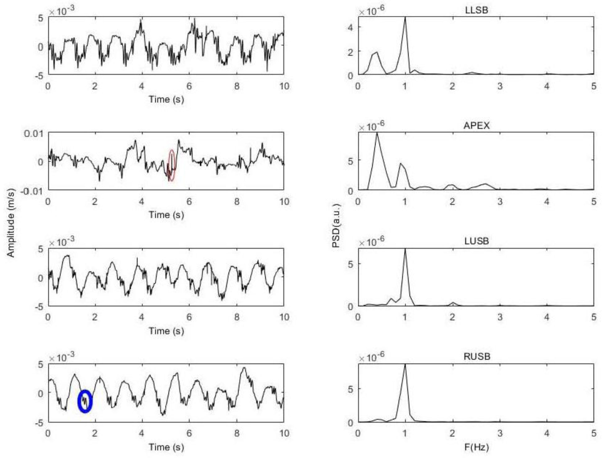
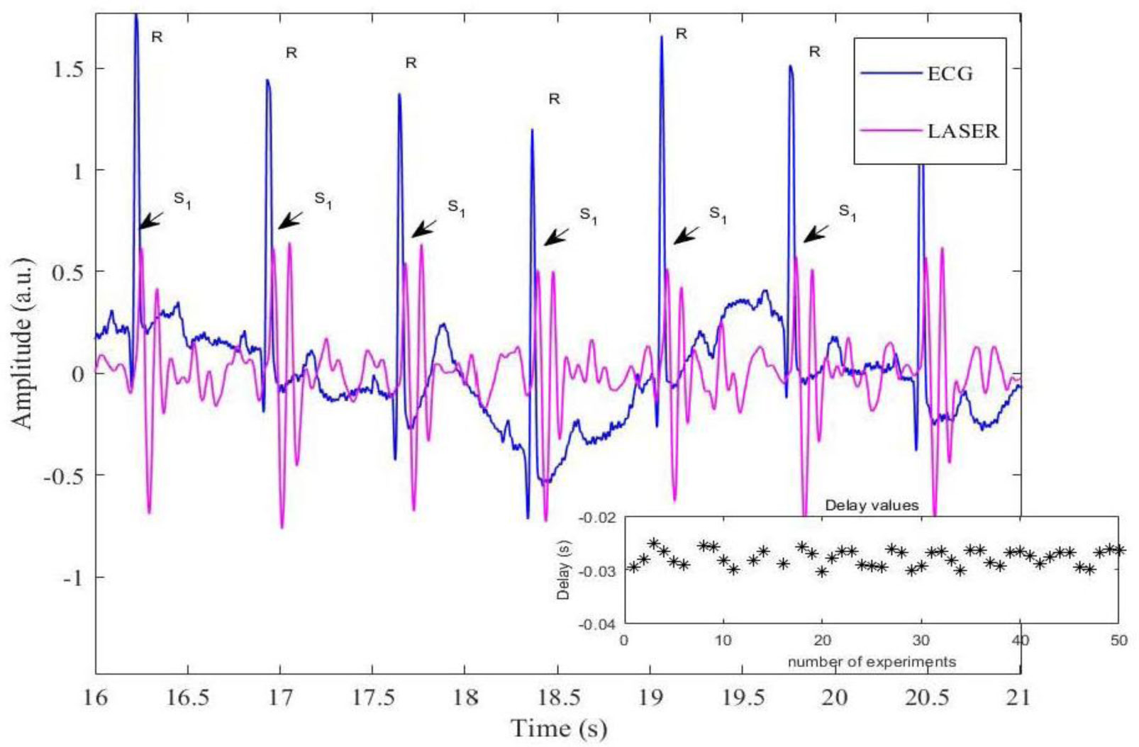
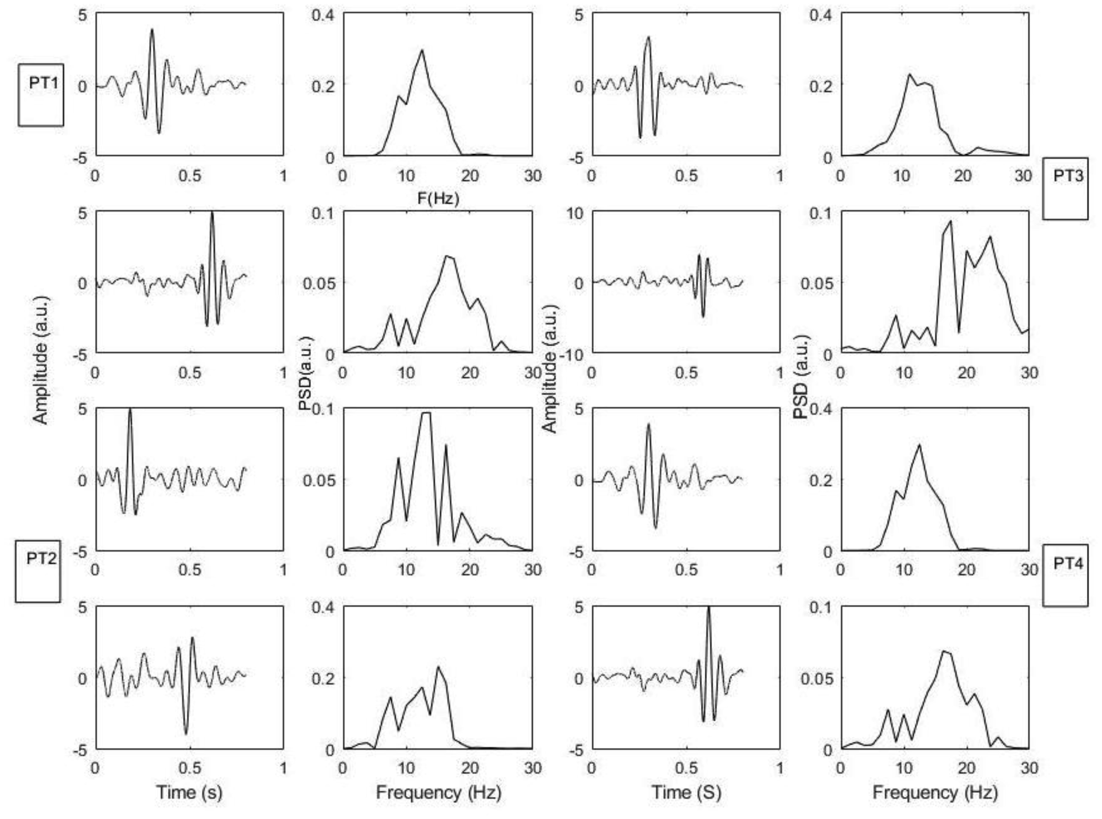
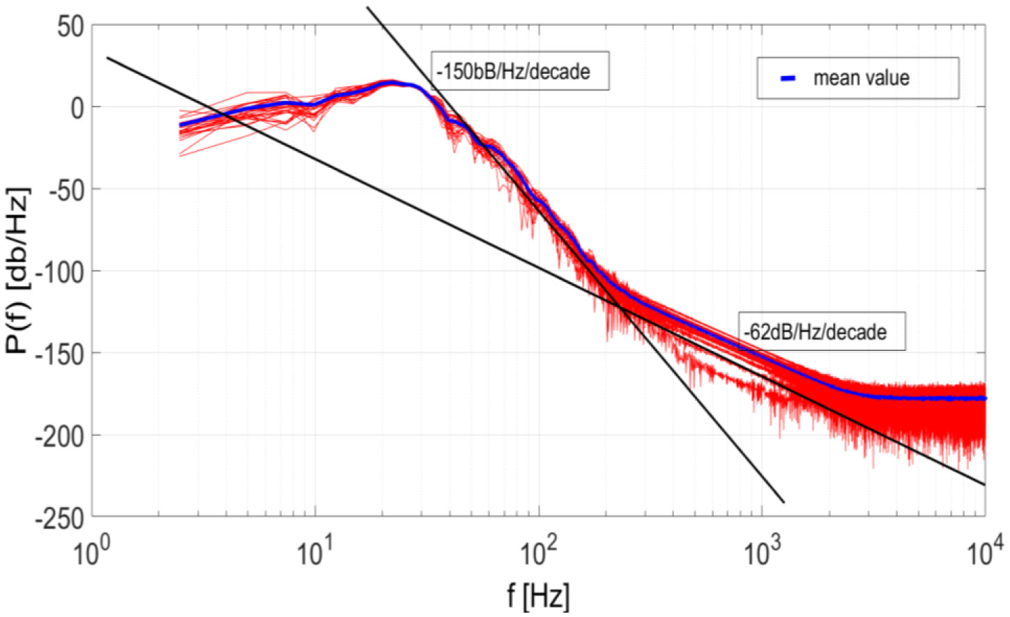
    [73] De Lauro E, De Martino S (2019) On the heart vibrations: Some insights from ECG and laser doppler vibrometry.p. atticon11705 V-C-5in press.
    [74] Scalise L (2012) Non contact heart monitoring. Advances in Electrocardiograms-Methods and Analysis Rijeka, Croatia: InTech, 81-106.
    [75] Tomasini E, Pinotti M, Paone N (1998) Carotid artery pulse wave measured by a laser vibrometer.3411: 611-616.
    [76] Morbiducci U, Scalise L, De Melis M (2006) Optical vibrocardiography: a novel tool for optical monitoring of cardiac activity. Ann Biomed Eng 35: 45-58. doi: 10.1007/s10439-006-9202-9
    [77] Buccheri G, De Lauro E, De Martino S, et al. (2016) Experimental study of self-oscillations of the trachea–larynx tract by laser doppler vibrometry. Biomed Phys Eng Express 2: 055009. doi: 10.1088/2057-1976/2/5/055009
    [78] Tavakolian K, Dumont GA, Blaber AP (2012) Analysis of seismocardiogram capability for trending stroke volume changes: A lower body negative pressure study. Computing in Cardiology 2012: 733-736.
    [79] Desjardins CL, Antonelli LT (2007) A remote and non-contact method for obtaining the blood pulse waveform with a laser Doppler vibrometer. Advanced Biomedical and Clinical Diagnostic Systems V, Proc. SPIE .
    [80] Hyvärinen A, Karhunen J, Oja E (2001)  Independent Component Analysis Hoboken, USA: John Wiley & Sons. doi: 10.1002/0471221317
    [81] Capuano P, De Lauro E, De Martino S, et al. (2017) Convolutive independent component analysis for processing massive datasets: a case study at Campi Flegrei (Italy). Nat Hazards 86: 417-429. doi: 10.1007/s11069-016-2545-0
    [82] Capuano P, De Lauro E, De Martino S (2016) Detailed investigation of long-period activity at Campi Flegrei by convolutive independent component analysis. Phys Earth Planet Inter 253: 48-57. doi: 10.1016/j.pepi.2016.02.003
    [83] Capuano P, De Lauro E, De Martino S (2011) Water-level oscillations in the Adriatic Sea as coherent self-oscillations inferred by independent component analysis. Prog Oceanogr 91: 447-460. doi: 10.1016/j.pocean.2011.06.001
    [84] De Lauro E, De Martino S, Falanga M, et al. (2006) Statistical analysis of Stromboli VLP tremor in the band [0.1–0.5] Hz: some consequences for vibrating structures. Nonlinear Process Geophys 13: 393-400. doi: 10.5194/npg-13-393-2006
    [85] Rüssel IK, Götte MJW, Bronzwaer JG, et al. (2009) Left ventricular torsion: an expanding role in the analysis of myocardial dysfunction. JACC Cardiovasc Imaging 2: 648-655. doi: 10.1016/j.jcmg.2009.03.001
    [86] Loppini A, Capolupo A, Cherubini C (2012) On the coherent behavior of pancreatic beta cell clusters. Phys Lett A 378: 3210-3217. doi: 10.1016/j.physleta.2014.09.041
    [87] Dal Lin C, Brugnolo L, Marinova M, et al. (2020) Toward a unified view of cognitive and biochemical activity: Meditation and linguistic self-reconstructing may lead to inflammation and oxidative stress improvement. Entropy 22: 818. doi: 10.3390/e22080818
    [88] Dal Lin C, Radu CM, Vitiello G, et al. (2020) In vitro effects on cellular shaping, contratility, cytoskeletal organization and mitochondrial activity in HL1 cells after different sounds stimulation. A qualitative pilot study and a theoretical physical model, 2020.
    [89] McFadden J, Al-Khalili J (2014)  Life on the edge: the coming of age of quantum biology London: Bantam Press.
    [90] McFadden J, Al-Khalili J (1999) A quantum mechanical model of adaptive mutation. Biosystems 50: 203-211. doi: 10.1016/S0303-2647(99)00004-0
    [91] Misra B, Sudarshan ECG (1977) The Zeno's paradox in quantum theory. J Math Phys 18: 756-763. doi: 10.1063/1.523304
    [92] Kraus K (1981) Measuring processes in quantum mechanics I. Continuous observation and the watchdog effect. Found Phys 11: 547-576. doi: 10.1007/BF00726936
    [93] Meloni M (2014) The social brain meets the reactive genome: neuroscience, epigenetics and the new social biology. Front Hum Neurosci 8: 309. doi: 10.3389/fnhum.2014.00309
    [94] Vitiello G (2014) On the isomorphism between dissipative systems, fractal self-similarity and electrodynamics. Toward an integrated vision of nature. Systems 2: 203-216. doi: 10.3390/systems2020203
    [95] Novack DH, Cameron O, Epel E, et al. (2007) Psychosomatic medicine: The scientific foundation of the biopsychosocial model. Acad Psychiatry 31: 388-401. doi: 10.1176/appi.ap.31.5.388
    [96] Dal Lin C, Gola E, Brocca A, et al. (2018) miRNAs may change rapidly with thoughts: The relaxation response after myocardial infarction. Eur J Integr Med 20: 63-72. doi: 10.1016/j.eujim.2018.03.009
    [97] Chrousos GP (2009) Stress and disorders of the stress system. Nat Rev Endocrinol 5: 374-381. doi: 10.1038/nrendo.2009.106
    [98] Muehsam D, Ventura C (2014) Life rhythm as a symphony of oscillatory patterns: electromagnetic energy and sound vibration modulates gene expression for biological signaling and healing. Glob Adv Health Med 3: 40-55. doi: 10.7453/gahmj.2014.008
    [99] (2015)  Heart Beat Made Visible on CymaScope Avaibale from: https://www.youtube.com/watch?v=2kuY98F7o_0.
    [100] Ingber DE, Wang N, Stamenović D (2014) Tensegrity, cellular biophysics, and the mechanics of living systems. Rep Prog Phys 77: 046603. doi: 10.1088/0034-4885/77/4/046603
    [101] Wang N, Tytell JD, Ingber DE (2009) Mechanotransduction at a distance: Mechanically coupling the extracellular matrix with the nucleus. Nat Rev Mol Cell Biol 10: 75-82. doi: 10.1038/nrm2594
    [102] Martino F, Perestrelo AR, Vinarsky V, et al. (2018) Cellular mechanotransduction: from tension to function. Frony Physiol 9: 824. doi: 10.3389/fphys.2018.00824
    [103] Buxbaum O (2016)  Key Insights into Basic Mechanisms of Mental Activity Switzerland: Springer International Publishing. doi: 10.1007/978-3-319-29467-4
    [104] Jamieson JP, Crum AJ, Goyer JP, et al. (2018) Optimizing stress responses with reappraisal and mindset interventions: an integrated model. Anxiety, Stress, Coping 31: 245-261. doi: 10.1080/10615806.2018.1442615
    [105] Pulvermüller F (2013) How neurons make meaning: Brain mechanisms for embodied and abstract-symbolic semantics. Trends Cogn Sci 17: 458-470. doi: 10.1016/j.tics.2013.06.004
    [106] Segall JM, Allen EA, Jung RE, et al. (2012) Correspondence between structure and function in the human brain at rest. Front Neuroinform 6: 10. doi: 10.3389/fninf.2012.00010
    [107] Alexander-Bloch A, Shou H, Liu S, et al. (2018) On testing for spatial correspondence between maps of human brain structure and function. Neuroimage 178: 540-551. doi: 10.1016/j.neuroimage.2018.05.070
    [108] Rebollo I, Devauchelle AD, Béranger B, et al. (2018) Stomach-brain synchrony reveals a novel, delayed-connectivity resting-state network in humans. Elife 7: e33321. doi: 10.7554/eLife.33321
    [109] Ventura C (2017) Seeing cell biology with the eyes of physics. NanoWorld J 3: S1-S8.
    [110] Fredericks S, Saylor JR (2013)  Shape oscillation of a levitated drop in an acoustic field, 2013 Available from: arXiv:1310.2967.
    [111] Zhang CY, Wang Y, Schubert R, et al. (2016) Effect of audible sound on protein crystallization. Cryst Growth Des 16: 705-713. doi: 10.1021/acs.cgd.5b01268
    [112] Guo F, Li P, French JB, et al. (2015) Controlling cell–cell interactions using surface acoustic waves. Proc Natl Acad Sci 112: 43-48. doi: 10.1073/pnas.1422068112
    [113] Vogel V, Sheetz M (2006) Local force and geometry sensing regulate cell functions. Nat Rev Mol Cell Biol 7: 265-275. doi: 10.1038/nrm1890
    [114] Shaobin G, Wu Y, Li K, et al. (2010) A pilot study of the effect of audible sound on the growth of Escherichia coli. Colloid Surface B 78: 367-371. doi: 10.1016/j.colsurfb.2010.02.028
    [115] Gu SB, Yang B, Wu Y, et al. (2013) Growth and physiological characteristics of E. coli in response to the exposure of sound field. Pakistan J Biol Sci 16: 969-975. doi: 10.3923/pjbs.2013.969.975
    [116] Sahu S, Ghosh S, Fujita D, et al. (2014) Live visualizations of single isolated tubulin protein self-assembly via tunneling current: effect of electromagnetic pumping during spontaneous growth of microtubule. Sci Rep 4: 7303. doi: 10.1038/srep07303
    [117] Acbas G, Niessen KA, Snell EH, et al. (2014) Optical measurements of long-range protein vibrations. Nat Commun 5: 3076. doi: 10.1038/ncomms4076
    [118] Christians ES, Benjamin IJ (2012) Proteostasis and REDOX state in the heart. Am J Physiol Heart Circ Physiol 302: H24-H37. doi: 10.1152/ajpheart.00903.2011
    [119] Christians ES, Mustafi SB, Benjamin IJ (2014) Chaperones and cardiac misfolding protein diseases. Curr Protein Pept Sci 15: 189-204. doi: 10.2174/1389203715666140331111518
    [120] Naviaux RK (2014) Metabolic features of the cell danger response. Mitochondrion 16: 7-17. doi: 10.1016/j.mito.2013.08.006
    [121] Crum A, Zuckerman B (2017) Changing mindsets to enhance treatment effectiveness. J Am Med Assoc 317: 2063-2064. doi: 10.1001/jama.2017.4545
    [122] Maas C, Belgardt D, Han KL, et al. (2009) Synaptic activation modifies microtubules underlying transport of postsynaptic cargo. Proc Natl Acad Sci 106: 8731-8736. doi: 10.1073/pnas.0812391106
    [123] Lo LP, Liu SH, Chang YC (2007) Assembling microtubules disintegrate the postsynaptic density in vitro. Cell Motil Cytoskeleton 64: 6-18. doi: 10.1002/cm.20163
    [124] Arimura N, Kaibuchi K (2007) Neuronal polarity: From extracellular signals to intracellular mechanisms. Nat Rev Neurosci 8: 194-205. doi: 10.1038/nrn2056
    [125] Macario AJL, Conway de Macario E (2000) Stress and molecular chaperones in disease. Int J Clin Lab Res 30: 49-66. doi: 10.1007/s005990070016
    [126] Dal Lin C, Marinova M, Brugnolo L, et al. Rapid senectome and alternative splicing miRNAs changes with the relaxation response: A one year follow-up study, 2020 Available from: Preprints doi:10.20944/preprints202007.0268.v1.
    [127] Picard M, McManus MJ, Gray JD, et al. (2015) Mitochondrial functions modulate neuroendocrine, metabolic, inflammatory, and transcriptional responses to acute psychological stress. Proc Natl Acad Sci 112: E6614-E6623. doi: 10.1073/pnas.1515733112
    [128] Piattelli-Palmarini M, Vitiello G (2015) Linguistics and some aspects of its underlying dynamics. Biolinguistics 9: 96-115.
    [129] Mańka R, Ogrodnik B (1991) A model of soliton transport along microtubules. J Biol Phys 18: 85-189. doi: 10.1007/BF00417807
    [130] Kučera O, Havelka D (2012) Mechano-electrical vibrations of microtubules-Link to subcellular morphology. BioSystems 109: 346-355. doi: 10.1016/j.biosystems.2012.04.009
    [131] Benias PC, Wells RG, Sackey-Aboagye B, et al. (2018) Structure and distribution of an unrecognized interstitium in human tissues. Sci Rep 8: 4947. doi: 10.1038/s41598-018-23062-6
    [132] Brizhik L, Chiappini E, Stefanini P, et al. (2019) Modeling meridians within the quantum field theory. J Acupunct Meridian Stud 12: 29-36. doi: 10.1016/j.jams.2018.06.009
    [133] Bentov I (1977)  Stalking the wild pendulum Glasgow: William Collins Sons & Co. Ltd.
    [134] Pavanello S, Campisi m, Tona F, et al. (2019) Exploring epigenetic age in response to intensive relaxing training: A pilot study to slow down biological age. Int J Env Res Pub He 16: 3074. doi: 10.3390/ijerph16173074
    [135] Dal Lin C, Grasso R, Scordino A, et al. (2020)  Ph, electric conductivity and delayed luminescence changes in human sera of subjects undergoing the relaxation response: A pilot study Available from: doi:10.20944/PREPRINTS202004.0202.V1.
    [136] Cifra M, Brouder C, Nerudová M, et al. (2015) Biophotons, coherence and photocount statistics: A critical review. J Lumin 164: 38-51. doi: 10.1016/j.jlumin.2015.03.020
    [137] Boveris A, Cadenas E, Reiter R (1980) Organ chemiluminescence: noninvasive assay for oxidative radical reactions. Proc Natl Acad Sci 77: 347-351. doi: 10.1073/pnas.77.1.347
    [138] Krasovitski B, Frenkel V, Shoham S (2011) Intramembrane cavitation as a unifying mechanism for ultrasound-induced bioeffects. Proc Natl Acad Sci 108: 3258-3263. doi: 10.1073/pnas.1015771108
    [139] Brujan EA (2000) Collapse of cavitation bubbles in blood. Europhys Lett 50: 175. doi: 10.1209/epl/i2000-00251-7
    [140] Brennen CE (2015) Cavitation in medicine. Interface Focus 5: 20150022. doi: 10.1098/rsfs.2015.0022
    [141] Didenko YT, Suslick KS (2002) The energy efficiency of formation of photons radicals and ions during single-bubble cavitation. Nature 418: 394-397. doi: 10.1038/nature00895
    [142] Sabbadini SA, Vitiello G (2019) Entanglement and phase-mediated correlations in quantum field theory. Application to brain-mind states. Appl Sci 9: 3203. doi: 10.3390/app9153203
    [143] Shaffer F, McCraty R, Zerr CL (2014) A healthy heart is not a metronome: an integrative review of the heart's anatomy and heart rate variability. Front Psychol 5: 1040. doi: 10.3389/fpsyg.2014.01040
    [144] Grippo A (2011) The utility of animal models in understanding links between psychosocial processes and cardiovascular health. Soc Pers Psychol Compass 5: 164-179. doi: 10.1111/j.1751-9004.2011.00342.x
    [145] Mensah G, Collins P (2015) Understanding mental health for the prevention and control of cardiovascular diseases. Glob Heart 10: 221. doi: 10.1016/j.gheart.2015.08.003
  • This article has been cited by:

    1. Zhifang Li, Huihong Zhao, Yunlong Shang, State estimation for censored system with colored noises: system reconstruction approach, 2022, 2183, 1742-6588, 012015, 10.1088/1742-6596/2183/1/012015
    2. Hassan Okasha, Yuhlong Lio, Mohammed Albassam, On Reliability Estimation of Lomax Distribution under Adaptive Type-I Progressive Hybrid Censoring Scheme, 2021, 9, 2227-7390, 2903, 10.3390/math9222903
    3. Mazen Nassar, Refah Alotaibi, Ahmed Elshahhat, Complexity Analysis of E-Bayesian Estimation under Type-II Censoring with Application to Organ Transplant Blood Data, 2022, 14, 2073-8994, 1308, 10.3390/sym14071308
    4. Refah Alotaibi, Mazen Nassar, Ahmed Elshahhat, Computational Analysis of XLindley Parameters Using Adaptive Type-II Progressive Hybrid Censoring with Applications in Chemical Engineering, 2022, 10, 2227-7390, 3355, 10.3390/math10183355
    5. Majd Alslman, Amal Helu, Lili Yu, Estimation of the stress-strength reliability for the inverse Weibull distribution under adaptive type-II progressive hybrid censoring, 2022, 17, 1932-6203, e0277514, 10.1371/journal.pone.0277514
    6. Zhifang Li, Huihong Zhao, Hailong Meng, Yong Chen, Variable step size predictor design for a class of linear discrete-time censored system, 2021, 6, 2473-6988, 10581, 10.3934/math.2021614
    7. Heba S. Mohammed, Empirical E-Bayesian estimation for the parameter of Poisson distribution, 2021, 6, 2473-6988, 8205, 10.3934/math.2021475
    8. Ahmed Elshahhat, Mazen Nassar, Inference of improved adaptive progressively censored competing risks data for Weibull lifetime models, 2023, 0932-5026, 10.1007/s00362-023-01417-0
    9. Monthira Duangsaphon, Sukit Sokampang, Kannat Na Bangchang, Bayesian estimation for median discrete Weibull regression model, 2024, 9, 2473-6988, 270, 10.3934/math.2024016
    10. 莉 张, Bayesian Analysis of Chen Distributionunder Improved Adaptive ProgressiveType-II Censoring, 2024, 14, 2160-7583, 400, 10.12677/PM.2024.141040
    11. Yarong Yu, Liang Wang, Sanku Dey, Jia Liu, Estimation of stress-strength reliability from unit-Burr Ⅲ distribution under records data, 2023, 20, 1551-0018, 12360, 10.3934/mbe.2023550
  • Reader Comments
  • © 2021 the Author(s), licensee AIMS Press. This is an open access article distributed under the terms of the Creative Commons Attribution License (http://creativecommons.org/licenses/by/4.0)
通讯作者: 陈斌, bchen63@163.com
  • 1. 

    沈阳化工大学材料科学与工程学院 沈阳 110142

  1. 本站搜索
  2. 百度学术搜索
  3. 万方数据库搜索
  4. CNKI搜索

Metrics

Article views(7604) PDF downloads(436) Cited by(0)

Figures and Tables

Figures(7)

/

DownLoad:  Full-Size Img  PowerPoint
Return
Return

Catalog