A new variant of estimation approach to asymmetric stochastic volatilitymodel

1.   Introduction

Consider a non trivial group $A$ and take an element $t$ not in $A$. Consider an equation,

where, $a_{j} \; \epsilon \; A$, $p_{j}$ = $\pm1$ and $a_{j} \; \neq$ 1 if it appears between two cyclically adjacent $t$ having exponents with different signs. The equation $s(t) = 1$ is solvable over the group $A$ if it has a solution in some group extension of $A$. Precisely, let $G$ be a group containing $A$, if there exist an injective homomorphism, say $\lambda: A \rightarrow G$, such that, $g_{1}g^{p_1}g_{2}g^{p_2} \cdots g_{n}g^{p_n} = 1$ in $G$, where $g_j = \lambda(a_j)$ and $g \in G$ then the equation $s(t) = 1$ is solvable over $A$. A conjecture stated in ^[2] by Levin asserts that if $A$ is torsion- free, then every equation over $A$ is solvable. Bibi and Edjvet ^[1], using in particular results of Prishchepov ^[3], has shown that the conjecture is true for equations of length at most seven. Here we prove the following: Theorem: The singular equation,

of length eight is solvable over any torsion-free group.

Levin showed that any equation over a torsion-free group is solvable if the exponent sum $p_{1} + p_{2} \cdots + p_{n}$ is same as length of the equation. Stallings proved that any equation of the form $a_{1}ta_{2}t \cdots a_{m}tb_{1}t^{-1}b_{2}t^{-1} \cdots b_{n}t^{-1} = 1$, is solvable over torsion-free group. Klyachko showed that any equation with exponent sum $\pm1$ is solvable over torsion free group.

2.   Preliminaries

All necessary definitions concerning relative presentations and pictures can be found in ^[4]. A relative group presentation $\textbf{P}$ is a triplet $< A, t|r >$ where $A$ is a group, $t$ is disjoint from $A$ and $\textbf{r}$ is a set of cyclically reduced words in $A\ast < t >$. If the relative presentation $\textbf{P}$ is orientable and aspherical then the natural homomorphism $A \rightarrow G$ is injective. $\textbf{P}$ is orientable and aspherical implies $s(t) = 1$ is solvable. We use $weight test$ to establish asphericity. The star graph $\Gamma$ of a relative presentation $\textbf{P} = < A, t| r >$ is a directed graph with vertex set $\{t, t^{-1}\}$ and edges set $r^{\ast}$, the set of all cyclic permutations of elements of $\{r, r^{-1}\}$ which begin with $t$ or $t^{-1}$. $\mathit{S} \; \in \; r^{\ast}$ write $\mathit{S} = \mathit{T}\alpha_{j}$ where $\alpha_{j} \; \in \; A$ and $\mathit{T}$ begins and ends with $t$ or $t^{-1}$. The initial function $\mathit{i}(\mathit{S})$ is the inverse of last symbol of $\mathit{T}$ and terminal function $\tau(\mathit{S})$ is the first symbol of $\mathit{T}$. The labeling function on the edges is defined by $\pi(\mathit{S}) = \alpha_{j}$ and is extended to paths in the usual way. A weight function $\theta$ on the star graph $\Gamma$ is a real valued function given to the edges of $\Gamma$. If $d$ is an edge of $\Gamma$, then $\theta(d)$ = $\theta(\bar{d})$. A weight function $\theta$ is aspherical if the following three conditions are satisfied:

(1) Let R $\epsilon \; \textbf{r}$ be cyclically reduced word, say $R = t_{1}^{\epsilon_{1}}a_{1}...t_{n}^{\epsilon_{n}}a_{n}$, where $\epsilon_{i}$ = $\pm1$ and $a_{i} \; \in$ A. Then,

(2) Each admissible cycle in $\Gamma$ has weight at least 2.

(3) Each edge of $\Gamma$ has a non-negative weight.

The relative presentation $\textbf{P}$ is aspherical if $\Gamma$ admits an aspherical weight function. For convenience we write $s(t) = 1$ as,

where $a, b, c, e, f, g \in A/\{1\}$ and $d, h \in A$. Moreover, by applying the transformation $y = td$, if necessary, it can be assumed without any loss that $d = 1$ in $A$.

3.   Key observations

(1) Since c(2, 2, 3, 3, 3, 3, 3, 3) = 0, so at least 3 admissible cycles must be of order 2.

(2) $ac$ and a$c^{-1}$ implies $c^{2}$ = 1, a contradiction.

(3) $af$ and a$f^{-1}$ implies $f^{2}$ = 1, a contradiction.

(4) $be$ and b$e^{-1}$ implies $e^{2}$ = 1, a contradiction.

(5) $bg$ and b$g^{-1}$ implies $g^{2}$ = 1, a contradiction.

(6) If two of $ac$, $af$ and c$f^{-1}$ are admissible then so is the third.

(7) If two of a$c^{-1}$, a$f^{-1}$ and c$f^{-1}$ are admissible then so is the third.

(8) If two of $ac, cf$ and a$f^{-1}$ are admissible then so is the third.

(9) If two of a$c^{-1}$, $af$ and $cf$ are admissible then so is the third.

(10) If two of $be, eg$, b$g^{-1}$ are admissible then so is the third.

(11) If two of b$e^{-1}$, $eg$ and $bg$ are admissible then so is the third.

4.   Cases

(1) $a = c^{-1}, b = e^{-1}$

(2) $a = c^{-1}, b = g^{-1}$

(3) $a = c^{-1}, e = g^{-1}$

(4) $a = c^{-1}, d = h^{-1}$

(5) $a = c^{-1}, b = e$

(6) $a = c^{-1}, b = g$

(7) $a = c, b = g^{-1}$

(8) $a = c, e = g^{-1}$

(9) $a = c, d = h^{-1}$

(10) $a = c, b = e$

(11) $a = c, b = g$

(12) $a = c, e = g$

(13) $a = f^{-1}, b = g^{-1}$

(14) $a = f^{-1}, d = h^{-1}$

(15) $a = f^{-1}, b = g$

(16) $c = f^{-1}, b = e^{-1}$

(17) $c = f^{-1}, b = g^{-1}$

(18) $c = f^{-1}, d = h^{-1}$

(19) $c = f^{-1}, b = e$

(20) $c = f^{-1}, b = g$

(21) $c = f^{-1}, e = g$

(22) $a = f, d = h^{-1}$

(23) $a = f, b = e$

(24) $a = f, b = g$

(25) $c = f, b = g^{-1}$

(26) $c = f, e = g^{-1}$

(27) $c = f, d = h^{-1}$

(28) $c = f, b = e$

(29) $b = e, d = h^{-1}$

(30) $a = c^{-1}, a = f^{-1}, d = h^{-1}$

(31) $a = c^{-1}, a = f^{-1}, c = f$

(32) $a = c^{-1}, a = f, c = f^{-1}$

(33) $a = c^{-1}, c = f^{-1}, d = h^{-1}$

(34) $a = c^{-1}, c = f, d = h^{-1}$

(35) $a = c, a = f, c = f$

(36) $a = c, a = f^{-1}, c = f^{-1}$

(37) $a = f^{-1}, c = f^{-1}, d = h^{-1}$

(38) $a = f^{-1}, c = f, d = h^{-1}$

(39) $a = f, c = f^{-1}, d = h^{-1}$

(40) $a = f, c = f, d = h^{-1}$

(41) $b = e^{-1}, b = g^{-1}, d = h^{-1}$

(42) $b = e^{-1}, b = g^{-1}, e = g$

(43) $b = e, b = g^{-1}, e = g^{-1}$

(44) $b = e^{-1}, b = g, e = g^{-1}$

(45) $b = e^{-1}, b = g, d = h^{-1}$

(46) $b = g^{-1}, e = g^{-1}, d = h^{-1}$

(47) $b = g^{-1}, e = g, d = h^{-1}$

(48) $b = g, e = g^{-1}, d = h^{-1}$

(49) $b = g, e = g, d = h^{-1}$

(50) $a = c^{-1}, a = f, c = f^{-1}, d = h^{-1}$

(51) $a = c^{-1}, a = f^{-1}, c = f, d = h^{-1}$

(52) $a = c^{-1}, b = e, b = g^{-1}, d = h^{-1}$

(53) $a = c, a = f^{-1}, c = f^{-1}, d = h^{-1}$

(54) $a = c, a = f, c = f, d = h^{-1}$

(55) $b = e^{-1}, b = g^{-1}, e = g, d = h^{-1}$

(56) $a = c^{-1}, b = e, b = g^{-1}, e = g^{-1}, d = h^{-1}$

(57) $a = c, a = f, c = f, b = e^{-1}, d = h^{-1}$

(58) $a = c, a = f, c = f, b = e, d = h^{-1}$

(59) $c = f, b = e, b = g^{-1}, e = g^{-1}, d = h^{-1}$

(60) $a = c, a = f^{-1}, c = f^{-1}, b = e^{-1}, b = g^{-1}, d = h^{-1}$

(61) $a = c, a = f, c = f, b = e^{-1}, b = g^{-1}, d = h^{-1}$

(62) $a = f^{-1}, c = f, b = e^{-1}, b = g, e = g^{-1}, d = h^{-1}$

(63) $a = f, c = f^{-1}, b = e, b = g^{-1}, e = g^{-1}, d = h^{-1}$

(64) $a = f, c = f^{-1}, b = e^{-1}, b = g, e = g^{-1}, d = h^{-1}$

(65) $a = c^{-1}, a = f, c = f^{-1}, b = e, b = g^{-1}, e = g^{-1}, d = h^{-1}$

(66) $a = c^{-1}, a = f^{-1}, c = f, b = e^{-1}, b = g, e = g^{-1}, d = h^{-1}$

(67) $a = c, a = f, c = f, b = e^{-1}, b = g, e = g^{-1}, d = h^{-1}$

5.   Proof of theorem

Recall that $\textbf{P} = < A, t|s(t) > = 1$ where $s(t) = atbt^{-1}ctdtet^{-1}ftgt^{-1}ht^{-1} = 1$ and $a, b, c, e, f, g \in A/\{1\}$ and $d, h \in A$. We will show that some cases of the given equation are solvable by applying the weight test. Also the transformation $y = td$, leads to the assumption that $d = 1$ in A.

5.1.   Case 1: $a = c^{-1}$, $b = e^{-1}$

In this case the relative presentation $\textbf{P}$ is given as :

$\textbf{P} = < A, t|s(t) = atbt^{-1}ctdtet^{-1}ftgt^{-1}ht^{-1} >$

= $< A, t|s(t) = c^{-1}te^{-1}t^{-1}ct^{2}et^{-1}ftgt^{-1}ht^{-1} = 1 >$.

Suppose, $x = tet^{-1}$ which implies that $x^{-1} = te^{-1}t^{-1}$.

Using above substitutions in relative presentation we have new presentation

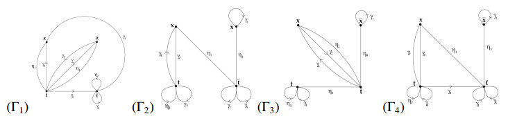
$\textbf{Q} = < A, t, x|t^{-1}c^{-1}x^{-1}ctxftgt^{-1}h = 1 = x^{-1}tet^{-1} >$. Observe that in new presentation $\textbf{Q}$ we have two relators $R_1 = t^{-1}c^{-1}x^{-1}ctxftgt^{-1}h$ and $R_2 = x^{-1}tet^{-1}$. The star graph $\Gamma_1$ for new presentation $\textbf{Q}$ is given by the Figure 1.

Let $\gamma_1 \leftrightarrow c^{-1}, \gamma_2 \leftrightarrow c, \gamma_3 \leftrightarrow 1, \gamma_4 \leftrightarrow f, \gamma_5 \leftrightarrow g, \gamma_6 \leftrightarrow h$ and $\eta_1 \leftrightarrow 1, \eta_2 \leftrightarrow e, \eta_3 \leftrightarrow 1$.

Assign weights to the edges of the star graph $\Gamma_1$ as follows:

$\theta(\gamma_1) = \theta(\gamma_2) = \theta(\eta_2) = 1$ and $\theta(\gamma_3) = \theta(\gamma_4) = \theta(\gamma_5) = \theta(\gamma_5) = \theta(\gamma_6) = \theta(\eta_1) = \theta(\eta_3) = \frac{1}{2}$. The given weight function $\theta$ is aspherical and all three conditions of weight test are satisfied.

(1) Observe that, $\sum (1-\theta(\gamma_j)) = 6 - (1 + 1 + \frac{1}{2} + \frac{1}{2} + \frac{1}{2}) + \frac{1}{2}) = 2$ and $\sum (1-\theta(\eta_j)) = 3 - (0 + 1 + 0) = 2$.

(2) Each admissible cycle having weight less than 2 leads to a contraction. For example, $\gamma_3\gamma_6\eta_1$ is a cycle of length 2 having weight less than 2, which implies $h = 1$, a contradiction.

(3) Each edge has non-negative weight.

5.2.   Case 2: $a = c^{-1}$, $b = g^{-1}$

In this case we have two relators $R_1 = t^{-1}atbt^{-1}a^{-1}t^{2}et^{-1}ftb^{-1}t^{-1}h$ and $R_2 = ta^{-1}t^{-1}$. The star graph $\Gamma_2$ for new presentation $\textbf{Q}$ is given by the Figure 1.

(1) Observe that, $\sum (1-\theta(\gamma_j)) = 6 - (0 + 1 + 1 + \frac{1}{2} + 1 + \frac{1}{2}) = 2$ and $\sum (1-\theta(\eta_j)) = 3 - (0 + 1 + 1) = 2$.

(2) Each admissible cycle having weight less than 2 leads to a contradiction. For example $\gamma_6\gamma_3\eta_1$ is a cycle of length 2, having weight less than 2, which implies $h = 1$, a contradiction.

(3) Each edge has non-negative weight.

5.3.   Case 3: $a = c^{-1}, e = g^{-1}$

In this case we have two relators $R_1 = xbx^{-1}tg^{-1}t^{-1}ftgt^{-1}h$ and $R_2 = x^{-1}t^{-1}at$. The star graph $\Gamma_2$ for new presentation $\textbf{Q}$ is given by the Figure 1.

(1) Observe that, $\sum (1-\theta(\gamma_j)) = 6 - (0 + 1 + 1 + \frac{1}{2} + 1 + \frac{1}{2}) = 2$ and $\sum (1-\theta(\eta_j)) = 3 - (0 + 1 + 0) = 2$.

(2) Each admissible cycle having weight less than 2 leads to a contradiction. For example, $\gamma_5\eta_3\gamma_1\eta_3$ is a cycles of length 2 having weight less than 2, which implies $b = g^{-1}$, a contradiction.

(3) Each admissible cycle has non-negative weight.

5.4.   Case 4: $a = c^{-1}, d = h^{-1}$

In this case we have two relators $R_1 = xbx^{-1}et^{-1}ftg$ and $R_2 = t^{-1}a^{-1}t^{2}$. The star graph $\Gamma_3$ for the relative presentation is given by the Figure 1.

(1) Observe that $\sum (1-\theta(\gamma_j)) = 4 - (0 + 1 + \frac{1}{2} + \frac{1}{2}) = 2$ and $\sum (1-\theta(\eta_j)) = 4 - (0 + \frac{1}{2} + 1 + \frac{1}{2}) = 2$.

(2) Each possible admissible cycle has weight atleast 2, so $\theta$ admits an aspherical weight function.

(3) Each edge has non-negative weight.

5.5.   Case 5: $a = c^{-1}, b = e$

In this case we have two relators $R_1 = xbx^{-1}tbt^{-1}ftgt^{-1}ht^{-1}$ and $R_2 = x^{-1}t^{-1}at$. The star graph $\Gamma_4$ for the relative presentation is given by the Figure 1.

(1) Observe that $\sum (1-\theta(\gamma_j)) = 7 - (0 + 1 + 1 + 1 + \frac{1}{2} + \frac{1}{2} + 1) = 2$ and $\sum (1-\theta(\eta_j)) = 3 - (0 + \frac{1}{2} + 1 + \frac{1}{2}) = 2$.

(2) Each admissible cycle having weight less than 2 leads to a contradiction. For example, $\gamma_5\eta_3\gamma_1\eta_3$ is a cycle of length 2 having weight less than 2, which implies $g = b^{-1}$ a contradiction.

(3) Each edge has non-negative weight.

5.6.   Case 6: $a = c^{-1}$, $b = g$

In this case we have two relators $R_1 = t^{-1}axa^{-1}t^{2}et^{-1}fxh$ and $R_2 = x^{-1}tb^{-1}t^{-1}$. The star graph $\Gamma_5$ for the relative presentation $\textbf{Q}$ is given by the Figure 2.

(1) Observe that, $\sum (1-\theta(\gamma_j)) = 6 - (\frac{1}{2} + 1 + \frac{1}{2} + 1 + \frac{1}{2} + \frac{1}{2}) = 2$ and $\sum (1-\theta(\eta_j)) = 3 - (\frac{1}{2} + \frac{1}{2} + 0) = 2$.

(2) Each admissible cycle having weight less than 2 leads to a contradiction. For example, $\gamma_6\gamma_3\eta_3$ is a cycle of length 2 having weight less than 2, which implies $h = 1$, a contradiction.

(3) Each edge has non-negative weight,

5.7.   Case 7: $a = c, b = g^{-1}$

In this case we have two relators $R_1 = xg^{-1}xtet^{-1}ftgt^{-1}h$ and $R_2 = x^{-1}t^{-1}ct$. The star graph $\Gamma_6$ for the relative presentation is given by the Figure 2.

(1) Observe that, $\sum (1-\theta(\gamma_j)) = 6 - (\frac{3}{2} + \frac{1}{2} + 1 + \frac{1}{2} + \frac{1}{2} + 0) = 2$ and $\sum (1-\theta(\eta_j)) = 3 - (0 + 1 + 0) = 2$

(2) Each admissible cycle having weight less than 2 leads to a contradiction, For example, the cycle $\gamma_1\eta_1\eta_3$, $\gamma_6\eta_1\eta_3\gamma_2$ and $\gamma_6\eta_1\eta_3\gamma_1$ are the cycles of length 2 having weight less than 2, which implies $g = 1$, $h = 1$ and $h = g$, a contradiction.

(3) Each edge has non-negative weight.

5.8.   Case 8: $a = c$, $e = g^{-1}$

In this case we have two relators $R_1 = xht^{-1}atbt^{-1}atx^{-1}f$ and $R_2 = x^{-1}tgt^{-1}$. The star graph $\Gamma_7$ for the relative presentation $\textbf{Q}$ is given by the Figure 2.

(1) Observe that, $\sum (1-\theta(\gamma_j)) = 6 - (\frac{1}{2} + 1 + 1 + 1 + \frac{1}{2} + 0) = 2$ and $\sum (1-\theta(\eta_j)) = 3 - (\frac{1}{2} + \frac{1}{2} + 0) = 2$.

(2) Each possible admissible cycle having weight less than 2 leads to a contradiction. For Example $\eta_2\gamma_5\gamma_1$ is a cycle of length 2 having weight less than 2, which implies $g = h^{-1}$, a contradiction.

(3) Each edge has non-negative weight.

5.9.   Case 9: $a = c, d = h^{-1}$

In this case we have two relators $R_1 = t^{-1}xbxtet^{-1}ftg$ and $R_2 = x^{-1}t^{-1}at$. The star graph $\Gamma_8$ for the relative presentation is given by the Figure 2.

(1) Observe that, $\sum (1-\theta(\gamma_j)) = 6 - (\frac{1}{2} + \frac{3}{2} + 0 + \frac{1}{2} + \frac{1}{2} + 1) = 2$ and $\sum (1-\theta(\eta_j)) = 3 - (0 + 1 + 0) = 2$.

(2) Each edge having weight less than 2 leads to a contradiction. For example, $\gamma_2\eta_1\eta_3$ is a cycle of length 2 having weight less than 2, which implies $b = 1$, a contradiction.

(3) Each edge has non-negative weight.

5.10.   Case 10: $a = c$. $b = e$

In this case we have two relators $R_1 = t^{-1}axatxftgt^{-1}h$ and $R_2 = x^{-1}tb^{-1}t^{-1}$. The star graph $\Gamma_{9}$ for the relative presentation is given by the Figure 3.

(1) Observe that, $\sum (1-\theta(\gamma_j)) = 6 - (1 + \frac{1}{2} + \frac{1}{2} + \frac{1}{2} + 1 + \frac{1}{2}) = 2$ and $\sum (1-\theta(\eta_j)) = 3 - (0 + \frac{1}{2} + \frac{1}{2}) = 2$.

(2) Each edge having weight less than 2 leads to a contradiction. For example, $\gamma_6\gamma_5\eta_1$ is a cycles of length 2 having weight less than 2, which implies that $h = 1$, a contradiction.

(3) Each edge has non-negative weight.

5.11.   Case 11: $a = c, b = g$

In this case we have two relators $R_1 = t^{-1}axat^{2}et^{-1}fxh$ and $R_2 = x^{-1}tgt^{-1}$. The star graph $\Gamma_{10}$ for the relative presentation is given by the Figure 3.

(1) Observe that, $\sum (1-\theta(\gamma_j)) = 6 - (\frac{1}{2} + 1 + \frac{1}{2} + 1 + \frac{1}{2} + \frac{1}{2}) = 2$ and $\sum (1-\theta(\eta_j)) = 3 - (\frac{1}{2} + \frac{1}{2} + 0) = 2$.

(2) Each edge having weight less than 2 leads to a contradiction. For example, $\gamma_6\gamma_3\eta_3$ is a cycles of length 2 having weight less than 2, which implies that $h = 1$, a contradiction.

(3) Each edge has non-negative weight.

5.12.   Case 12: $a = c, e = g$

In this case we have two relators $R_1 = t^{-1}ctbt^{-1}axfx^{-1}th$ and $R_2 = x^{-1}t^{2}et^{-1}$. The star graph $\Gamma_{11}$ for the relative presentation is given by the Figure 3.

(1) Observe that $\sum (1-\theta(\gamma_j)) = 6 - (1 + \frac{1}{2} + 0 + \frac{1}{2} + 1 + 1) = 2$ and $\sum (1-\theta(\eta_j)) = 4 - (1 + 0 + \frac{1}{2} + \frac{1}{2}) = 2$.

(2) Each possible admissible cycle has weight atleast 2, so $\theta$ admits an aspherical weight function.

(3) Each edge has non-negative weight.

5.13.   Case 13: $a = f^{-1}$, $b = g^{-1}$

In this case we have two relators $R_1 = xbt^{-1}ct^{2}ex^{-1}b^{-1}t^{-1}h$ and $R_2 = x^{-1}t^{-1}at$. The star graph $\Gamma_{12}$ for the relative presentation is given by the Figure 3.

(1) Observe that, $\sum (1-\theta(\gamma_j)) = {6 - (\frac{1}{2} + \frac{1}{2} + 0 + 1 + 1 + 1}) = 2$ and $\sum (1-\theta(\eta_j)) = 3 - (0 + 1 + 0) = 2$.

(2) Each edge having weight less than 2 leads to a contradiction. For example, $\gamma_6\gamma_3\eta_1$ is a cycles of length 2 having weight less than 2, which implies that $h = 1$, a contradiction.

(3) Each edge has non negative weight.

5.14.   Case 14: $a = f^{-1}$, $d = h^{-1}$

In this case we have two relators $R_1 = t^{-1}xbt^{-1}ct^{2}exg$ and $R_2 = x^{-1}t^{-1}ft$. The star graph $\Gamma_{13}$ for the relative presentation is given by the Figure 4.

(1) $\sum (1-\theta(\gamma_j)) = 6 - (\frac{1}{2} + \frac{1}{2} + 1 + 1 + 1 + 0) = 2$ and $\sum (1-\theta(\eta_j)) = 3 - (0 + \frac{1}{2} + \frac{1}{2}) = 2$.

(2) Each edge having weight less than 2 leads to a contradiction. For example, $\gamma_6\gamma_4\gamma_1$ amd $\gamma_6\gamma_5\eta_1\eta_3$ are the cycles of length 2 having weight less than 2, which implies $g = 1$ and $g = e^{-1}$, a contradiction.

(3) Each edge has non-negative weight.

5.15.   Case 15: $a = f^{-1}$, $b = g$

In this case we have two relators $R_1 = xbt^{-1}ct^{2}ex^{-1}bt^{-1}h$ and $R_2 = x^{-1}t^{-1}at$. The star graph $\Gamma_{13}$ for the relative presentation Q is given by the Figure 4.

(1) Observe that, $\sum (1-\theta(\gamma_j)) = {6 - (\frac{1}{2} + 1 + 1 + \frac{1}{2} + 1 + 0}) = 2$ and $\sum (1-\theta(\eta_j)) = {3 - (0 + \frac{1}{2} + \frac{1}{2}}) = 2$.

(2) Each admissible cycle having weight less than 2 leads to a contradiction. For example, $\gamma_6\eta_1\gamma_3$ is a cycle of length 2 having weight less than 2, which implies $h = 1$, a contradiction.

(3) Each edge has non-negative weight.

5.16.   Case 16: $c = f^{-1}$, $b = e^{-1}$

In this case we have two relators $R_1 = t^{-1}ac^{-1}tx^{-1}ctxgt^{-1}h$ and $R_2 = x^{-1}tb^{-1}t^{-1}c^{-1}t$. The star graph $\Gamma_{14}$ for the relative presentation $\textbf{Q}$ is given by the Figure 4.

(1) Observe that, $\sum (1-\theta(\gamma_j)) = 6 - (1 + \frac{1}{2} + 1 + 1 + \frac{1}{2} + 0) = 2$ and $\sum (1-\theta(\eta_j)) = 4 - (0 + 1 + \frac{1}{2} + \frac{1}{2}) = 2$.

(2) Each admissible cycle having weight less than 2 leads to a contradiction. For example, $\gamma_6\eta_1\gamma_4$ is a cycles of length 2, having weight less than 2, which implies $h = 1$ a contradiction.

(3) Each edge has non-negative weight.

5.17.   Case 17: $c = f^{-1}$, $b = g^{-1}$

In this case we have two relators $R_1 = t^{-1}axtex^{-1}h$ and $R_2 = x^{-1}tbt^{-1}ct$. The star graph $\Gamma_{15}$ for the relative presentation $\textbf{Q}$ is given by the Figure 4.

(1) Observe that, $\sum (1-\theta(\gamma_j)) = 4 - (1 + 0 + 1 + 0) = 2$ and $\sum (1-\theta(\eta_j)) = 4 - (1 + 0 + 0 + 1) = 2$.

(2) Each admissible cycle having weight less than 2 leads to a contradiction. For example, $\gamma_4\eta_4\gamma_2\gamma_1$ is a cycle of length 2 having weight less than 2, which implies $h = 1$, a contradiction.

(3) Each edge has non-negative weight.

5.18.   Case 18: $c = f^{-1}$, $d = h^{-1}$

In this case we have two relators $R_1 = t^{-2}atbx^{-1}texg$ and $R_2 = x^{-1}t^{-1}et^{-1}c^{-1}t$. The star graph $\Gamma_{16}$ for the relative presentation Q is given by the Figure 4.

(1) $\sum (1-\theta(\gamma_j)) = 4 - (1 + 1 + \frac{1}{2} + \frac{1}{2} + \frac{1}{2}) = 2$ and $\sum (1-\theta(\eta_j)) = 4 - (\frac{1}{2} + \frac{1}{2} + \frac{1}{2} + \frac{1}{2}) = 2$.

(2) Each admissible cycle has weight atleast 2, so $\theta$ admits an aspherical weight function.

(3) Each edge has non-negative weight.

5.19.   Case 19: $c = f^{-1}$, $b = e$

In this case we have two relators $R_1 = t^{-1}atbxtbx^{-1}gt^{-1}h$ and $R_2 = x^{-1}t^{-1}ct$. The star graph $\Gamma_{17}$ for the relative presentation $\textbf{Q}$ is given by the Figure 5.

(1) $\sum (1-\theta(\gamma_j)) = 6 - (1 + \frac{1}{2} + 1 + \frac{1}{2} + 1 + \frac{1}{2} + \frac{1}{2}) = 2$ and $\sum (1-\theta(\eta_j)) = 3 - (\frac{1}{2} + \frac{1}{2} + 0) = 2$.

(2) Each admissible cycle having weight less than 2 leads to a contradiction. For example, $\gamma_6\eta_3\gamma_3$ is a cycle of length 2 having weight less than 2, which implies $h = 1$, a contradiction.

(3) Each edge has non-negative weight.

5.20.   Case 20: $c = f^{-1}$, $b = g$

In this case we have two relators $R_1 = t^{-1}axct^{2}et^{-1}c^{-1}tbt^{-1}h$ and $R_2 = x^{-1}tbt^{-1}$. The star graph $\Gamma_{18}$ for the relative presentation $\textbf{Q}$ is given by the Figure 5.

(1) Observe that, $\sum (1-\theta(\gamma_j)) = 6 - (\frac{1}{2} + 1 + \frac{1}{2} + 1 + \frac{1}{2} + \frac{1}{2}) = 2$ and $\sum (1-\theta(\eta_j)) = 3 - (\frac{1}{2} + \frac{1}{2} + 0) = 2$.

(2) Each admissible cycle having weight less than 2 leads to a contradiction. For example, $\gamma_6\gamma_3\eta_3$ is a cycle of length 2 having weight less than 2, which implies $h = 1$ a contradiction.

(3) Each edge has non-negative weight.

5.21.   Case 21: $c = f^{-1}$, $e = g$

In this case we have two relators $R_1 = t^{-1}atbxtex^{-1}et^{-1}h$ and $R_2 = x^{-1}t^{-1}ct$. The star graph $\Gamma_{19}$ for the relative presentation $\textbf{Q}$ is given by the Figure 5.

(1) Observe that, $\sum (1-\theta(\gamma_j)) = 6 - (\frac{1}{2} + 1 + \frac{1}{2} + 1 + \frac{1}{2} + \frac{1}{2}) = 2$ and $\sum (1-\theta(\eta_j)) = 3 - (0 + 1 + 0) = 2$.

(2) Each admissible cycle having weight less than 2 leads to a contradiction. For example, $\gamma_6\eta_3\gamma_3$ is a cycle of length 2 having weight less than 2, which implies $h = 1,$ a contradiction.

(3) Each edge has non-negative weight.

5.22.   Case 22: $a = f$, $d = h^{-1}$

In this case we have two relators $R_1 = t^{-1}xbt^{-1}ct^{2}exg$ and $R_2 = x^{-1}t^{-1}at$. The star graph $\Gamma_{20}$ for the $\textbf{Q}$ relative presentation is given by the Figure 5.

(1) Observe that, $\sum (1-\theta(\gamma_j)) = 6 - (1 + \frac{1}{2} + 1 + 1 +0 + \frac{1}{2}) = 2$ and $\sum (1-\theta(\eta_j)) = 3 - (0 + \frac{1}{2} + \frac{1}{2}) = 2$.

(2) Each possible admissible cycle has weight atleast 2, so $\theta$ admits an aspherical weight function.

(3) Each edge has non-negative weight.

5.23.   Case 23: $a = f, b = e$

In this case we have two relators $R_1 = t^{-1}axctxatget^{-1}h$ and $R_2 = x^{-1}tbt^{-1}$.

The star graph $\Gamma_{21}$ for the relative presentation $\textbf{Q}$ is given by the Figure 6.

(1) Observe that, $\sum (1-\theta(\gamma_j)) = 6 - (\frac{1}{2} + \frac{1}{2} + 1 + \frac{1}{2} + \frac{1}{2} + 1) = 2$ and $\sum (1-\theta(\eta_j)) = 3 - (0 + \frac{1}{2} + \frac{1}{2}) = 2$.

(2) Each admissible cycle having weight less than 2 leads to a contradiction. For example, $\gamma_6\gamma_3\eta_1$, is a cycle of length 2 having weight less than 2, which implies $h = 1$ a contradiction.

(3) Each edge has non-negative weight.

5.24.   Case 24: $a = f, b = g$

In this case we have two relators $R_1 = xct^{2}exh$ and $R_2 = x^{-1}t^{-1}atbt^{-1}$. The star graph $\Gamma_{22}$ for the relative presentation $\textbf{Q}$ is given by the Figure 6.

(1) Observe that, $\sum (1-\theta(\gamma_j)) = 4 - (\frac{1}{2} + \frac{1}{2} + \frac{1}{2} + \frac{1}{2}) = 2$ and $\sum (1-\theta(\eta_j)) = 4 - (\frac{1}{2} + \frac{1}{2} + \frac{1}{2} + \frac{1}{2}) = 2$.

(2) Each admissible cycle having weight less than 2 leads to a contradiction. For example, $\gamma_3^{2}\eta_1$ is a cycle of length 2, having weight less than 2, which implies $e^{2} = 1$, a contradiction.

(3) Each edge has non-negative weight.

5.25.   Case 25: $c = f$, $b = g^{-1}$

In this case we have two relators $R_1 = t^{-1}atg^{-1}xtexgt^{-1}h$ and $R_2 = x^{-1}t^{-1}ft >$. The star graph $\Gamma_{23}$ for the relative presentation is given by the Figure 6.

(1) Observe that, $\sum (1-\theta(\gamma_j)) = 6 - (1 + \frac{1}{2} + \frac{1}{2} + \frac{1}{2} + 1 + \frac{1}{2}) = 2$ and $\sum (1-\theta(\eta_j)) = 3 - (\frac{1}{2} + \frac{1}{2} + 0) = 2$.

(2) Each admissible cycle having weight less than 2 leads to a contradiction. For example, $\gamma_6\eta_3\gamma_3$ is a cycle of length 2 having weight less than 2, which implies $h = 1$, a contradiction.

(3) Each edge has non-negative weight.

5.26.   Case 26: $c = f$, $e = g^{-1}$

In this case we have two relators $R_1 = t^{-1}atbxtexe^{-1}t^{-1}h$ and $R_2 = x^{-1}t^{-1}ct$. The star graph $\Gamma_{23}$ for the relative presentation Q is given by the Figure 6.

(1) Observe that, $\sum (1-\theta(\gamma_j)) = 6 - (1 + \frac{1}{2} + \frac{1}{2} + \frac{1}{2} + 1 + \frac{1}{2}) = 2$ and $\sum (1-\theta(\eta_j)) = 3 - (\frac{1}{2} + \frac{1}{2} + 0) = 2$.

(2) Each admissible cycle having weight less than 2 leads to a contradiction. For example, $\gamma_6\eta_3\gamma_3$ has weight less than 2, which implies $h = 1$, a contradiction.

(3) Each edge has non-negative weight.

5.27.   Case 27: $c = f$, $d = h^{-1}$

In this case we have two relators $R_1 = t^{-2}atbxtexg$ and $R_2 = x^{-1}t^{-1}ct$. The star graph $\Gamma_{24}$ for the relative presentation $\textbf{Q}$ is given by the Figure 6.

(1) Observe that, $\sum (1-\theta(\gamma_j)) = 6 - (1 + \frac{1}{2} + 1 + 1 + \frac{1}{2} + 0) = 2$ and $\sum (1-\theta(\eta_j)) = 3 - (0 + 1 + 0) = 2$.

(2) Each possible admissible cycle has weight at least 2, so $\theta$ admits an aspherical weight function.

(3) Each edge has non-negative weight.

5.28.   Case 28: $c = f, b = e$

In this case we have two relators $R_1 = t^{-1}axt^{-1}cxctgt^{-1}h$ and $R_2 = x^{-1}t^{2}bt^{-1}$. The star graph $\Gamma_{25}$ for the relative presentation $\textbf{Q}$ is given by the Figure 7.

(1) $\sum (1-\theta(\gamma_j)) = 4 - (\frac{1}{2} + \frac{1}{2} + \frac{1}{2} + \frac{1}{2}) = 2$ and $\sum (1-\theta(\eta_j)) = 4 - (\frac{1}{2} + \frac{1}{2} + \frac{1}{2} + \frac{1}{2}) = 2$.

(2) Each possible admissible cycle has weight atleast 2, so $\theta$ admits an aspherical weight function.

(3) Each edge has non-negative weight.

6.   Case 29: $b = e$, $d = h^{-1}$

In this case we have two relators $R_1 = xcta^{-1}t^{2}xftg$ and $R_2 = x^{-1}t^{-2}atbt^{-1}$. The star graph $\Gamma_{26}$ for the relative presentation $\textbf{Q}$ is given by the Figure 7.

(1) $\sum (1-\theta(\gamma_j)) = 6 - (1 + \frac{1}{2} + 1 + \frac{1}{2} + \frac{1}{2} + \frac{1}{2}) = 2$ and $\sum (1-\theta(\eta_j)) = 5 - (\frac{1}{2} + 1 + \frac{1}{2} + \frac{1}{2} + \frac{1}{2}) = 2$.

(2) Each possible admissible cycle has weight atleast 2, so $\theta$ admits an aspherical weight function.

(3) Each edge has non-negative weight.

6.1.   Case 30: $a = c^{-1}$, $a = f^{-1}$, $d = h^{-1}$

In this case we have two relators $R_1 = t^{-1}xbx^{-1}tex^{-1}g$ and $R_2 = x^{-1}t^{-1}at$. The star graph $\Gamma_{27}$ for the relative presentation $\textbf{Q}$ is given by the Figure 7.

(1) $\sum (1-\theta(\gamma_j)) = 5 - (1 + 0 + 1 + 1 + 0) = 2$ and $\sum (1-\theta(\eta_j)) = 3 - (0 + 0 + 1) = 2$.

(2) Each possible admissible cycle has weight atleast 2, so $\theta$ admits an aspherical weight function.

(3) Each edge has non-negative weight.

6.2.   Case 51: $a = c^{-1}$, $a = f^{-1}$, $c = f$, $d = h^{-1}$

In this case we have two relators $R_1 = t^{-1}axctx^{-1}fte^{-1}t^{-1}h$ and $R_2 = x^{-1}tbt^{-1}$. The star graph $\Gamma_{27}$ for the new presentation $\textbf{Q}$ is given by the Figure 7.

(1) Observe that, $\sum (1-\theta(\gamma_j)) = 5 - (1 + 0 + 1 + 1 + 0) = 2$ and $\sum (1-\theta(\eta_j)) = 3 - (0 + 0 + 1) = 2$.

(2) Each possible admissible cycle has weight atleast 2 so $\theta$ admits an aspherical weight function.

(3) Each edge has non-negative weight.

6.3.   Case 31: $a = c^{-1}$, $a = f^{-1}$, $c = f$

In this case we have two relators $R_1 = xbx^{-1}tex^{-1}gt^{-1}h$ and $R_2 = x^{-1}t^{-1}at$. The star graph $\Gamma_{27}$ for the relative presentation $\textbf{Q}$ is given by the Figure 7.

(1) Observe that, $\sum (1-\theta(\gamma_j)) = 5 - (0 + 1 + 1 + 0 + 1) = 2$ and $\sum (1-\theta(\eta_j)) = 3 - (0 + 0 + 1) = 2$.

(2) Each possible admissible cycle has weight atleast 2, so $\theta$ admits an aspherical weight function.

(3) Each edge has non-negative watch.

6.4.   Case 32: $a = c^{-1}$, $a = f$, $c = f^{-1}$

In this case we have two relators: $R_1 = xbx^{-1}tet^{-1}c^{-1}tgt^{-1}h$ and $R_2 = x^{-1}t^{-1}at$. The star graph $\Gamma_{28}$ for the relative presentation $\textbf{Q}$ is given by the Figure 7.

(1) Observe that, $\sum (1-\theta(\gamma_j)) = 5 - (0 + 1 + 1 + 1 + \frac{1}{2} + \frac{1}{2}) = 2$ and $\sum (1-\theta(\eta_j)) = 3 - (0 + \frac{1}{2} + \frac{1}{2}) = 2$.

(2) Each possible admissible cycle having weight less than 2 leads to a contrdiction. For example, $\gamma_5\eta_3\gamma_1$ is a cycle of length 2 having weight less than 2, which implies $g = b^{-1}$, a contradiction.

(3) Each edge has non-negative weight.

6.5.   Case 33: $a = c^{-1}$, $c = f^{-1}$, $d = h^{-1}$

In this case we have two relators $R_1 = t^{-1}xbx^{-1}texg$ and $R_2 = x^{-1}t^{-1}at$. The star graph $\Gamma_{29}$ for the relative presentation $\textbf{Q}$ is given by the Figure 8.

(1) Observe that, $\sum (1-\theta(\gamma_j)) = 5 - (1 + 0 + 1 + 0 + 1) = 2$ and $\sum (1-\theta(\eta_j)) = 3 - (0 + 0 + 1) = 2$.

(2) Each possible admissible cycle has weight atleast 2, so $\theta$ admits an aspherical weight function.

(3) Each edge has non-negative weight.

6.6.   Case 34: $a = c^{-1}$, $c = f$, $d = h^{-1}$

In this case we have two relators $R_1 = t^{-1}xbx^{-1}tex^{-1}g$ and $R_2 = x^{-1}t^{-1}at$. The star graph $\Gamma_{30}$ for the relative presentation $\textbf{Q}$ is given by the Figure 8.

(1) Observe that, $\sum (1-\theta(\gamma_j)) = 5 - (1 + 0 + 1 + 1 + 0) = 2$ and $\sum (1-\theta(\eta_j)) = 3 - (0 + 0 + 1) = 2$.

(2) Each possible admissible cycle has weight atleast 2, so $\theta$ admits an aspherical weight function.

(3) Each edge has non-negative weight.

6.7.   Case 35: $a = c, a = f, c = f$

In this case we have two relators $R_1 = xbxtexgt^{-1}h$ and $R_2 = x^{-1}t^{-1}at$. The star graph $\Gamma_{31}$ for the relative presentation $\textbf{Q}$ is given by the Figure 8.

(1) Observe that, $\sum (1-\theta(\gamma_j)) = 5 - (1 + 0 + \frac{1}{2} + \frac{1}{2} + 1) = 2$ and $\sum (1-\theta(\eta_j)) = 3 - (\frac{1}{2} + 0 + \frac{1}{2}) = 2$.

(2) Each possible admissible cycle has weight atleast 2, so $\theta$ admits an aspherical weight function.

(3) Each edge has non-negative weight.

6.8.   Case 36: $a = c$, $a = f^{-1}$, $c = f^{-1}$

In this case we have two relators $R_1 = xbxtex^{-1}gt^{-1}h$ and $R_2 = x^{-1}t^{-1}at$. The star graph $\Gamma_{32}$ for the relative presentation $\textbf{Q}$ is given by the Figure 8.

(1) Observe that, $\sum (1-\theta(\gamma_j)) = 5 - (0 + 1 + 0 + 1 + 1) = 2$ and $\sum (1-\theta(\eta_j)) = 3 - (1 + 0 + 0) = 2$.

(2) Each possible admissible cycle has weight atleast 2, so $\theta$ admits an aspherical weight function.

(3) Each edge has non-negative weight.

6.9.   Case 37: $a = f^{-1}$, $c = f^{-1}$, $d = h^{-1}$

In this case we have two relators $R_1 = t^{-1}xbxtex^{-1}g$ and $R_2 = x^{-1}t^{-1}at$. The star graph $\Gamma_{33}$ for the relative presentation $\textbf{Q}$ is given by the Figure 9.

(1) Observe that $\sum (1-\theta(\gamma_j)) = 5 - (1 + 1 + 0 + \frac{1}{2} + \frac{1}{2}) = 2$ and $\sum (1-\theta(\eta_j)) = 3 - (\frac{1}{2} + 0 + \frac{1}{2}) = 2$.

(2) Each possible admissible cycle has weight atleast 2, so $\theta$ admits an aspherical weight function.

(3) Each edge has non-negative weight.

6.10.   Case 38: $a = f^{-1}$, $c = f$, $d = h^{-1}$

In this case we have two relators $R_1 = t^{-1}xbt^{-1}ct^{2}ex^{-1}g$ and $R_2 = x^{-1}t^{-1}at$. The star graph $\Gamma_{38}$ for the relative presentation $\textbf{Q}$ is given by the Figure 9.

(1) Observe that, $\sum (1-\theta(\gamma_j)) = 6 - (1 + \frac{1}{2} + 1 + 1 + \frac{1}{2} + 0) = 2$ and $\sum (1-\theta(\eta_j)) = 3 - (0 + \frac{1}{2} + \frac{1}{2}) = 2$.

(2) Each admissible cycle having weight less than 2 leads to a contradiction. For example, $\gamma_2\gamma_6^{-1}\eta_1\eta_3\gamma_5$ is the cycle of length 2 having weight less than 2, which leads to a contradiction.

(3) Each edge has non-negative weight.

6.11.   Case 39: $a = f$, $c = f^{-1}$, $d = h^{-1}$

In this case we have two relators $R_1 = t^{-1}xbx^{-1}texg$ and $R_2 = x^{-1}t^{-1}at$. The star graph $\Gamma_{35}$ for the relative presentation $\textbf{Q}$ is given by the Figure 9.

(1) Observe that, $\sum (1-\theta(\gamma_j)) = 5 - (0 + 1 + 1 + 1 + 0) = 2$ and $\sum (1-\theta(\eta_j)) = 3 - (1 + 0 + 0) = 2$.

(2) Each possible admissible cycle has weight atleast 2, so $\theta$ admits an aspherical weight function.

(3) Each edge has non-negative weight.

6.12.   Case 65: $a = c^{-1}$, $a = f$, $c = f^{-1}$, $b = e$, $b = g^{-1}$, $e = g^{-1}$, $d = h^{-1}$

In this case we have two relators $R_1 = t^{-1}xbx^{-1}tbxb^{-1}$ and $R_2 = x^{-1}t^{-1}at$. The star graph $\Gamma_{35}$ for the relative presentation $\textbf{Q}$ is given by the Figure 9.

(1) Observe that, $\sum (1-\theta(\gamma_j)) = 5 - (1 + 0 + 1 + 0 + 1) = 2$ and $\sum (1-\theta(\eta_j)) = 3 - (0 + 0 + 1) = 2$.

(2) Each possible admissible cycle has weight atleast 2 so $\theta$ admits an aspherical weight function.

(3) Each edge has non-negative weight.

6.13.   Case 40: $a = f$, $c = f$, $d = h^{-1}$

In this case we have two relators $R_1 = t^{-1}xbxtexg$ and $R_2 = x^{-1}t^{-1}at$. The star graph $\Gamma_{36}$ for the relative presentation $\textbf{Q}$ is given by the Figure 9.

(1) Observe that, $\sum (1-\theta(\gamma_j)) = 5 - (0 + 1 + 1 + 1 + 0) = 2$ and $\sum (1-\theta(\eta_j)) = 3 - (1 + 0 + 0) = 2$.

(2) Each possible admissible cycle has weight atleast 2, so $\theta$ admits an aspherical weight function.

(3) Each edge has non-negative weight.

6.14.   Case 41: $b = e^{-1}$, $b = g^{-1}$, $d = h^{-1}$

In this case we have two relators $R_1 = t^{-1}axctx^{-1}fx^{-1}$ and $R_2 = x^{-1}tbt^{-1}$. The star graph $\Gamma_{37}$ for the relative presentation $\textbf{Q}$ is given by the Figure 10.

(1) Observe that, $\sum (1-\theta(\gamma_j)) = 5 - (\frac{1}{2} + \frac{1}{2} + 1 + 1 + 0) = 2$ and $\sum (1-\theta(\eta_j)) = 3 - (\frac{1}{2} + \frac{1}{2} + 0) = 2$.

(2) Each possible admissible cycle has weight atleast 2, so $\theta$ admits an aspherical weight function.

(3) Each edge has non-negative weight.

6.15.   Case 42: $b = e^{-1}$, $b = g^{-1}$, $e = g$

In this case we have two relators $R_1 = t^{-1}axctx^{-1}fx^{-1}h$ and $R_2 = x^{-1}tbt^{-1}$. The star graph $\Gamma_{37}$ for the relative presentation $\textbf{Q}$ is given by the Figure 9.

(1) Observe that, $\sum (1-\theta(\gamma_j)) = 5 - (\frac{1}{2} + \frac{1}{2} + 1 + 1 + 0) = 2$ and $\sum (1-\theta(\eta_j)) = 3 - (\frac{1}{2} + 0 + \frac{1}{2}) = 2$.

(2) Each possible admissible cycle has weight atleast 2, so $\theta$ admits an aspherical weight function

(3) Each edge has non-negative weight.

6.16.   Case 43: $b = e$, $b = g^{-1}$, $e = g^{-1}$

In this case we have two relators $R_1 = t^{-1}axctxfx^{-1}h$ and $R_2 = x^{-1}tbt^{-1}$. The star graph $\Gamma_{38}$ for the relative presentation $\textbf{Q}$ is given by the Figure 10.

(1) Observe that, $\sum (1-\theta(\gamma_j)) = 5 - (0 + 1 + 1 + 0 + 1) = 2$ and $\sum (1-\theta(\eta_j)) = 3 - (0 + 0 + 1) = 2$.

(2) Each possible admissible cycle has weight atleast 2, so $\theta$ admits an aspherical weight function.

(3) Each edge has non-negative weight.

6.17.   Case 44: $b = e^{-1}$, $b = g$, $e = g^{-1}$

In this case we have two relators $R_1 = t^{-1}axctx^{-1}fte^{-1}t^{-1}h$ and $R_2 = x^{-1}tbt^{-1}$. The star graph $\Gamma_{39}$ for the relative presentation $\textbf{Q}$ is given by the Figure 10.

(1) Observe that, $\sum (1-\theta(\gamma_j)) = 6 - (\frac{1}{2} + 1 + 0 + \frac{1}{2} + 1 + 1) = 2$ and $\sum (1-\theta(\eta_j)) = 3 - (\frac{1}{2} + \frac{1}{2} + 0) = 2$.

(2) Each admissible cycle having weight less than 2 leads to a contradiction. For example, $\gamma_5\eta_1\eta_3$ is the cycle of length 2 having weight less than 2, which implies $h = 1$, a contradiction.

(3) Each edge has non-negative weight.

6.18.   Case 45: $b = e^{-1}$, $b = g$, $d = h^{-1}$

In this case we have two relators $R_1 = t^{-1}axctx^{-1}fx$ and $R_2 = x^{-1}tbt^{-1}$. The star graph $\Gamma_{40}$ for the relative presentation $\textbf{Q}$ is given by the Figure 10.

(1) Observe that, $\sum (1-\theta(\gamma_j)) = 6 - (\frac{1}{2} + 1 + 0 + \frac{1}{2} + 1 + 1) = 2$ and $\sum (1-\theta(\eta_j)) = 3 - (\frac{1}{2} + \frac{1}{2} + 0) = 2$.

(2) Each possible admissible cycle has weight atleast 2 so $\theta$ admits an aspherical weight function.

(3) Each edge has non-negative weight.

6.19.   Case 46: $b = g^{-1}$, $e = g^{-1}$, $d = h^{-1}$

In this case we have two relators $R_1 = |t^{-1}axctxfx^{-1}$ and $R_2 = x^{-1}tbt^{-1}$. The star graph $\Gamma_{41}$ for the relative presentation $\textbf{Q}$ is given by the Figure 11.

(1) Observe that, $\sum (1-\theta(\gamma_j)) = 6 - (\frac{1}{2} + 1 + 0 + \frac{1}{2} + 1 + 1) = 2$ and $\sum (1-\theta(\eta_j)) = 3 - (\frac{1}{2} + \frac{1}{2} + 0) = 2$.

(2) Each possible admissible cycle has weight atleast 2 so $\theta$ admits an aspherical weight function.

(3) Each edge has non-negative weight.

6.20.   Case 52: $a = c^{-1}$, $b = e$, $b = g^{-1}$, $d = h^{-1}$

In this case we have two relators $R_1 = t^{-1}axa^{-1}txfx^{-1}$ and $R_2 = x^{-1}tbt^{-1}$. The star graph $\Gamma_{41}$ for the relative presentation $\textbf{Q}$ is given by the Figure 11.

(1) Observe that, $\sum (1-\theta(\gamma_j)) = 5 - (0 + 1 + 1 + 0 + 1) = 2$ and $\sum (1-\theta(\eta_j)) = 3 - (0 + 0 + 1) = 2$.

(2) Each possible admissible cycle has weight atleast 2 so $\theta$ admits an aspherical weight function.

(3) Each edge has non-negative weight.

7.   Case 47: $b = g^{-1}$, $e = g$, $d = h^{-1}$

In this case we have two relators $R_1 = x^{-1}t^{-1}axctx^{-1}f$ and $R_2 = x^{-1}tbt^{-1}$. The star graph $\Gamma_{42}$ for the relative presentation $\textbf{Q}$ is given by the Figure 11.

(1) Observe that, $\sum (1-\theta(\gamma_j)) = 5 - (0 + \frac{1}{2} + \frac{1}{2} + 1 + 1) = 2$ and $\sum (1-\theta(\eta_j)) = 3 - (\frac{1}{2} + 0 + \frac{1}{2}) = 2$.

(2) Each admissible cycle has weight atleast 2 so $\theta$ admits an aspherical weight function.

(3) each edge has non-negative weight.

8.   Case 48: $b = g$, $e = g^{-1}$, $d = h^{-1}$

In this case we have two relators $R_1 = xatbt^{-1}cx^{-1}f$ and $R_2 = x^{-1}tbt^{-2}$. The star graph $\Gamma_{43}$ for the relative presentation $\textbf{Q}$ is given by the Figure 11.

(1) Observe that, $\sum (1-\theta(\gamma_j)) = 6 - (\frac{1}{2} + 1 + 0 + \frac{1}{2} + 1 + 1) = 2$ and $\sum (1-\theta(\eta_j)) = 3 - (\frac{1}{2} + \frac{1}{2} + 0) = 2$.

(2) Each possible admissible cycle has weight atleast 2 so $\theta$ admits an aspherical weight function.

(3) Each edge has non-negative weight.

9.   Case 49: $b = g$, $e = g$, $d = h^{-1}$

In this case we have two relators $R_1 = xt^{-1}axctxf$ and $R_2 = x^{-1}tbt^{-1}$. The star graph $\Gamma_{44}$ for the relative presentation $\textbf{Q}$ is given by the Figure 11.

(1) Observe that, $\sum (1-\theta(\gamma_j)) = 5 - (\frac{1}{2} + \frac{1}{2} + \frac{1}{2} + \frac{1}{2} + 1) = 2$ and $\sum (1-\theta(\eta_j)) = 3 - (\frac{1}{2} + 0 + \frac{1}{2}) = 2$.

(2) Each possible admissible cycle has weight atleast 2 so $\theta$ admits an aspherical weight function.

(3) Each edge has non-negative weight.

9.1.   Case 50: $a = c^{-1}$, $a = f$, $c = f^{-1}$, $d = h^{-1}$

In this case we have two relators $R_1 = xbx^{-1}etxg$ and $R_2 = x^{-1}t^{-2}c^{-1}t$. The star graph $\Gamma_{45}$ for the relative presentation $\textbf{Q}$ is given by the Figure 12.

(1) Observe that, $\sum (1-\theta(\gamma_j)) = 4 - (0 + 1 + 1 + 0) = 2$ and $\sum (1-\theta(\eta_j)) = 4 - (1 + 0 + 0 + 1) = 2$.

(2) Each possible admissible cycle has weight atleast 2 so $\theta$ admits an aspherical weight function.

(3) Each edge has non-negative weight.

9.2.   Case 53: $a = c$, $a = f^{-1}$, $c = f^{-1}$, $d = h^{-1}$

In this case we have two relators $R_1 = t^{-1}xbxtex^{-1}g$ and $R_2 = x^{-1}t^{-1}at$. The star graph $\Gamma_{46}$ for the relative presentation $\textbf{Q}$ is given by the Figure 12.

(1) Observe that, $\sum (1-\theta(\gamma_j)) = 5 - (1 + 1 + 0 + 0 + 1) = 2$ and $\sum (1-\theta(\eta_j)) = 3 - (1 + 0 + 0) = 2$.

(2) Each possible admissible cycle has weight atleast 2 so $\theta$ admits an aspherical weight function.

(3) Each edge has non-negative weight.

9.3.   Case 54: $a = c$, $a = f$, $c = f$, $d = h^{-1}$

In this case we have two relators $R_1 = t^{-1}xbxtexg$ and $R_2 = x^{-1}t^{-1}at$. The star graph $\Gamma_{47}$ for the relative presentation $\textbf{Q}$ is given by the Figure 12.

(1) Observe that, $\sum (1-\theta(\gamma_j)) = 5 - (1 + 1 + 0 + 1 + 0) = 2$ and $\sum (1-\theta(\eta_j)) = 3 - (1 + 0 + 0) = 2$.

(2) Each possible admissible cycle has weight atleast 2 so $\theta$ admits an aspherical weight function.

(3) Each edge has non-negative weight.

9.4.   Case 55: $b = e^{-1}$, $b = g^{-1}$, $e = g$, $d = h^{-1}$

In this case we have two relators $R_1 = x^{-1}t^{-1}axctx^{-1}f$ and $R_2 = x^{-1}tbt^{-1}$. The star graph $\Gamma_{48}$ for the relative presentation $\textbf{Q}$ is given by the Figure 12.

(1) Observe that, $\sum (1-\theta(\gamma_j)) = 5 - (0 + 0 + 1 + 1 + 1) = 2$ and $\sum (1-\theta(\eta_j)) = 3 - (0 + 0 + 0) = 2$.

(2) Each possible admissible cycle has weight atleast 2 so $\theta$ admits an aspherical weight function.

(3) Each edge has non-negative weight.

9.5.   Case 56: $a = c^{-1}$, $b = e$, $b = g^{-1}$, $e = g^{-1}$, $d = h^{-1}$

In this case we have two relators $R_1 = xc^{-1}x^{-1}tcx^{-1}f$ and $R_2 = x^{-1}tb^{-1}t^{-2}$. The star graph $\Gamma_{49}$ for the relative presentation $\textbf{Q}$ is given by the Figure 13.

(1) Observe that, $\sum (1-\theta(\gamma_j)) = 4 - (0 + 1 + 1 + 0) = 2$ and $\sum (1-\theta(\eta_j)) = 4 - (1 + 0 + 0 + 1) = 2$.

(2) Each possible admissible cycle has weight atleast 2 so $\theta$ admits an aspherical weight function.

(3) Each edge has non-negative weight.

9.6.   Case 57: $a = c$, $a = f$, $c = f$, $b = e^{-1}$, $d = h^{-1}$

In this case we have two relators $R_1 = t^{-1}xbxtb^{-1}xg$ and $R_2 = x^{-1}t^{-1}at$. The star graph $\Gamma_{50}$ for the relative presentation $\textbf{Q}$ is given by the Figure 13.

(1) Observe that, $\sum (1-\theta(\gamma_j)) = 5 - (\frac{1}{2} + 1 + \frac{1}{2} + 1 + 0) = 2$ and $\sum (1-\theta(\eta_j)) = 3 - (\frac{1}{2} + 0 + \frac{1}{2} = 2$.

(2) Each admissible cycle having weight less than 2 leads to a contradiction. For example $\gamma_2\eta_1\gamma_5^{-1}$ is a cycle of length 2 having weight less than 2 which implies $b = g$, a contradiction.

(3) Each edge has non-negative weight.

9.7.   Case 58: $a = c, a = f, c = f, b = e$, $d = h^{-1}$

In this case we have two relators $R_1 = |t^{-1}xbxtbxg$ and $R_2 = x^{-1}t^{-1}at$. The star graph $\Gamma_{50}$ for the relative presentation $\textbf{Q}$ is given by the Figure 12.

(1) Observe that, $\sum (1-\theta(\gamma_j)) = 5 - (\frac{1}{2} + 1 + \frac{1}{2} + 1 + 0) = 2$ and $\sum (1-\theta(\eta_j)) = 3 - (\frac{1}{2} + 0 + \frac{1}{2}) = 2$.

(2) Each admissible cycle having weight less than 2 leads to a contradiction. For example $\gamma_2\eta_1\gamma_5^{-1}$ is a cycle of length 2 having weight less than 2 which implies $b = g$, a contradiction.

(3) Each edge has non-negative weight.

9.8.   Case 59: $c = f, b = e$, $b = g^{-1}$, $e = g^{-1}$, $d = h^{-1}$

In this case we have two relators $R_1 = x^{-1}t^{-1}axctxc$ and $R_2 = x^{-1}tbt^{-1}$. The star graph $\Gamma_{51}$ for the relative presentation $\textbf{Q}$ is given by the Figure 13.

(1) Observe that, $\sum (1-\theta(\gamma_j)) = 5 - (1 + 0 + 0 + 1 + 1) = 2$ and $\sum (1-\theta(\eta_j)) = 3 - (0 + 0 + 1) = 2$.

(2) Each possible admissible cycle has weight atleast 2 so $\theta$ admits an aspherical weight function.

(3) Each edge has non-negative weight.

9.9.   Case 60: $a = c$, $a = f^{-1}$, $c = f^{-1}$, $b = e^{-1}$, $b = g^{-1}$, $d = h^{-1}$

In this case we have two relators $R_1 = xat^{-1}x^{-1}atxta^{-1}$ and $R_2 = x^{-1}tbt^{-1}t^{-2}$. The star graph $\Gamma_{52}$ for the relative presentation $\textbf{Q}$ is given by the Figure 13.

(1) Observe that, $\sum (1-\theta(\gamma_j)) = 6 - (0 + 1 + 0 + 1 + 1 + 1) = 2$ and $\sum (1-\theta(\eta_j)) = 4 - (0 + 0 + 1 + 1) = 2$.

(2) Each possible admissible cycle has weight atleast 2 so $\theta$ admits an aspherical weight function.

(3) Each edge has non-negative weight.

9.10.   Case 61: $a = c, a = f, c = f$, $b = e^{-1}$, $b = g^{-1}$, $d = h^{-1}$

In this case we have two relators $R_1 = t^{-1}xbxtb^{-1}xb^{-1}$ and $R_2 = x^{-1}t^{-1}at$. The star graph $\Gamma_{53}$ for the relative presentation $\textbf{Q}$ is given by the Figure 14.

(1) Observe that, $\sum (1-\theta(\gamma_j)) = 5 - (\frac{1}{2} + 1 + \frac{1}{2} + 1 + 0) = 2$ and $\sum (1-\theta(\eta_j)) = 3 - (\frac{1}{2} + 0 + \frac{1}{2}) = 2$.

(2) Each possible admissible cycle has weight atleast 2 so $\theta$ admits an aspherical weight function.

(3) Each edge has non-negative weight.

9.11.   Case 62: $a = f^{-1}$, $c = f$, $b = e^{-1}$, $b = g$, $e = g^{-1}$, $d = h^{-1}$

In this case we have two relators $R_1 = xbt^{-1}x^{-1}bxtb^{-1}tb^{-1}$ and $R_2 = x^{-1}t^{-1}a^{-1}tbt^{-1}$. The star graph $\Gamma_{54}$ for the relative presentation $\textbf{Q}$ is given by the Figure 14.

(1) Observe that, $\sum (1-\theta(\gamma_j)) = 6 - (\frac{1}{2} + 1 + 0 + 1 + \frac{1}{2} + 1) = 2$ and $\sum (1-\theta(\eta_j)) = 4 - (1 + 0 + 0 + 1) = 2$.

(2) Each possible admissible cycle has weight atleast 2 so $\theta$ admits an aspherical weight function.

(3) Each edge has non-negative weight.

9.12.   Case 63: $a = f$, $c = f^{-1}$, $b = e$, $b = g^{-1}$, $e = g^{-1}$, $d = h^{-1}$

In this case we have two relators $R_1 = t^{-1}axa^{-1}txax^{-1}$ and $R_2 = x^{-1}tbt^{-1}$. The star graph $\Gamma_{55}$ for the relative presentation $\textbf{Q}$ is given by the Figure 14.

(1) Observe that, $\sum (1-\theta(\gamma_j)) = 5 - (0 + 1 + 1 + 0 + 1) = 2$ and $\sum (1-\theta(\eta_j)) = 3 - (0 + 0 + 1) = 2$.

(2) Each possible admissible cycle has weight atleast 2 so $\theta$ admits an aspherical weight function.

(3) Each edge has non-negative weight.

9.13.   Case 64: $a = f$, $c = f^{-1}$, $b = e^{-1}$, $b = g$, $e = g^{-1}$, $d = h^{-1}$

In this case we have two relators $R_1 = t^{-1}xbx^{-1}tb^{-1}xb$ and $R_2 = x^{-1}t^{-1}at$. The star graph $\Gamma_{56}$ for the relative presentation $\textbf{Q}$ is given by the Figure 14.

(1) Observe that, $\sum (1-\theta(\gamma_j)) = 5 - (1 + 0 + 1 + 0 + 1) = 2$ and $\sum (1-\theta(\eta_j)) = 3 - (0 + 0 + 1) = 2$.

(2) Each possible admissible cycle has weight atleast 2 so $\theta$ admits an aspherical weight function.

(3) Each edge has non-negative weight.

9.14.   Case 66: $a = c^{-1}$, $a = f^{-1}$, $c = f$, $b = e^{-1}$, $b = g$, $e = g^{-1}$, $d = h^{-1}$

In this case we have two relators $R_1 = t^{-1}xbx^{-1}tb^{-1}x^{-1}b$ and $R_2 = x^{-1}t^{-1}at$. The star graph $\Gamma_{57}$ for the relative presentation $\textbf{Q}$ is given by the Figure 14.

(1) Observe that, $\sum (1-\theta(\gamma_j)) = 5 - (1 + 0 + 1 + 1 + 0) = 2$ and $\sum (1-\theta(\eta_j)) = 3 - (0 + 0 + 1) = 2$.

(2) Each possible admissible cycle has weight atleast 2 so $\theta$ admits an aspherical weight function.

(3) Each edge has non-negative weight.

9.15.   Case 67: $a = c$, $a = f$, $c = f$, $b = e^{-1}$, $b = g$, $e = g^{-1}$, $d = h^{-1}$

In this case we have two relators $R_1 = t^{-1}axatx^{-1}ax$ and $R_2 = x^{-1}tbt^{-1}$. The star graph $\Gamma_{58}$ for the relative presentation $\textbf{Q}$ is given by the Figure 15.

(1) Observe that, $\sum (1-\theta(\gamma_j)) = 5 - (1 + 0 + 1 + 0 + 1) = 2$ and $\sum (1-\theta(\eta_j)) = 3 - (1 + 0 + 0) = 2$.

(2) Each possible admissible cycle has weight atleast 2 so $\theta$ admits an aspherical weight function.

(3) Each edge has non-negative weight.

In all the cases, 3 conditions of weight test are satisfied.

Hence the equation $s(t) = atbt^{-1}ctdtet^{-1}ftgt^{-1}ht^{-1} = 1$ where $a, b, c, e, f, g \in A/\{1\}$ and $d, h \in A$ is solvable.

10.   Conclusions

In this article, we reviewed some basic concepts of combinatorial group theory (like torsion-free group, equations over groups, relative presentation, weight test) and discussed the two main conjectures in equations over torsion-free groups. We investigated all possible cases and solved the singular equation of length eight over torsion free group by using weight test. This result will be useful in dealing with equations over torsion-free groups.

Acknowledgments

The authors wish to express their gratitude to Prince Sultan University for facilitating the publication of this article through the Theoretical and Applied Sciences Lab.

Conflict of interest

All authors declare no conflicts of interest in this paper.