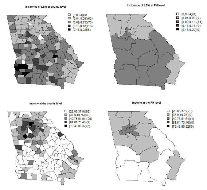
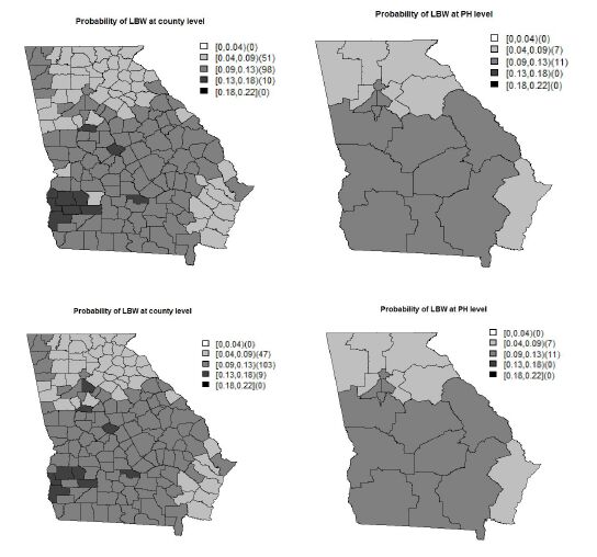
Low birth weight (LBW) is an important public health issue in the US as well as worldwide. The two main causes of LBW are premature birth and fetal growth restriction. Socio-economic status, as measured by family income has been correlated with LBW incidence at both the individual and population levels. In this paper, we investigate the impact of household income on LBW incidence at di erent geographical levels. To show this, we choose to examine LBW incidences collected from the state of Georgia, in the US, at both the county and public health (PH) district. The data at the PH district are an aggregation of the data at the county level nested within the PH district. A spatial scaling effect is induced during data aggregation from the county to the PH level. To address the scaling effect issue, we applied a shared multiscale model that jointly models the data at two levels via a shared correlated random effect. To assess the bene t of using the shared multiscale model, we compare it with an independent multiscale model which ignores the scale effect. Applying the shared multiscale model for the Georgia LBW incidence, we have found that income has a negative impact at both the county and PH levels. On the other hand, the independent multiscale model shows that income has a negative impact only at the county level. Hence, if the scale effect is not properly accommodated in the model, a different interpretation of the ndings could result.
Abbreviation: HR: Heart Rate; EDV: End Diastolic Volume; ESV: End Systolic Volume; CO: Cardiac Output; SV: Stroke Volume; EF: Ejection Fraction; DBP: (Systemic) Diastolic Blood Pressure; SBP: (Systemic) Systolic Blood Pressure; PAP: Pulmonary artery pressure
1.
Introduction
The Coronavirus disease 2019 (COVID-19) caused by the severe acute respiratory syndrome coronavirus 2 (SARS-CoV-2) primarily affects the respiratory system, although other organ systems are also involved and in particular cardiovascular complications may occur.
Among hospitalized patients with COVID-19, there is a high prevalence of previous history of cardiovascular diseases (CVD) and/or CVD risk factors; increased morbidity and mortality in those patients have been recently reported in several studies [1,2,3,4,5,6].
In particular, the COVID-19 infection can lead to myocarditis, vascular inflammation, arrhythmias, acute heart failure, and in the most severe cases, cardiogenic shock and death [1,2]. Studies of patients with COVID-19 in China indicated significantly higher in-hospital mortality rate in patients who also have myocardial injury. Acute infections increase the risk of acute coronary syndrome. COVID-19 may increase circulating cytokines, which have the potential to cause instability and rupture of atherosclerotic plaques. Moreover, some studies highlighted that, for patients hospitalized with COVID-19, a higher rate of comorbidities including hypertension and coronary artery disease characterized fatal events when compared to survivors [4] and myocardial injury was prevalent [5]. In any case, the interplay of COVID-19 with cardiovascular complications both in healthy individuals and in patients with pre-existing CVD is still far from being fully understood. The mechanisms of cardiac injury in patients with COVID-19 are not well established but it is reasonable to identify both direct and indirect mechanisms responsible for cardiac failure.
Possible causes of the effect of COVID-19 on cardiac impairment are due to an increased pulmonary vascular resistance consistent with severe inflammation and micro-thrombosis in the pulmonary microcirculation [7]. On the other side, the decreased blood saturation secondary to respiratory failure may hamper the cardiomyocytes contractility, possibly leading to a decreased cardiac output. Both as a compensatory mechanism for the reduced oxygen concentration in blood and consequence of fever rise due to the COVID-19 inflammation, the heart rate may significantly increase.
In this study, we provided examples of possible scenarios that reflect the effect of COVID-19 on some cardiac features of interest and other vital parameters. With this aim, we exploited the predictive nature of computational methods [8] that are based on the numerical solution (i.e., aided by a computer) of the mathematical equations underlying the physical processes under investigation. In this context, a zero-dimensional (0D, also known as lumped parameters) model that simulates systemic and pulmonary blood dynamics together with the cardiac function has been considered [9]. This tool can account for a broad range of the model parameters, to simulate variations in pulmonary resistances, heart rate, and cardiomyocyte contractility in accordance with COVID-19 infection, and to compute the corresponding changes of some meaningful outputs such as stroke volume, ejection fraction, cardiac output, arterial and pulmonary pressures. We studied the changes of heamodynamics indicators in the cardiac function associated with changes in heart rate, pulmonary resistance and ventricular contractility, which may be directly and indirectly associated to a COVID-19 infection. The use of a 0D mathematical model allowed us to better understand the strong interplay between local changes (such as the reduced contractility), global variables (such as peripheral resistances, heart rate) and cardiac function. This is of utmost importance in view of determining the possible effects of COVID-19 infection on patients already affected by CVD. A possible scenario of COVID-19 infection in a hypothetical individual exhibiting impaired ejection fraction and cardiac output is investigated to support the predictive power of our computational study and its possible exploitation for patient-specific studies.
This 0D analysis has also been complemented by a computational study carried out with a 3D-0D model. In this model, three-dimensional electro-mechanical activity of the LV is represented with a higher level of detail through a multiscale and multiphysics model, accounting for cardiac electrophysiology, the microscopic generation of active force, and tissue mechanics. This represents a starting point for possible developments of the study here conducted, which may include the customization of the analysis through the use of cardiac models tailored on the specific patient.
2.
Models and methods
2.1. The zero-dimensional (0D) computational model
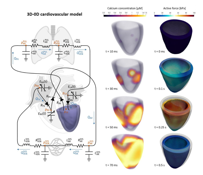
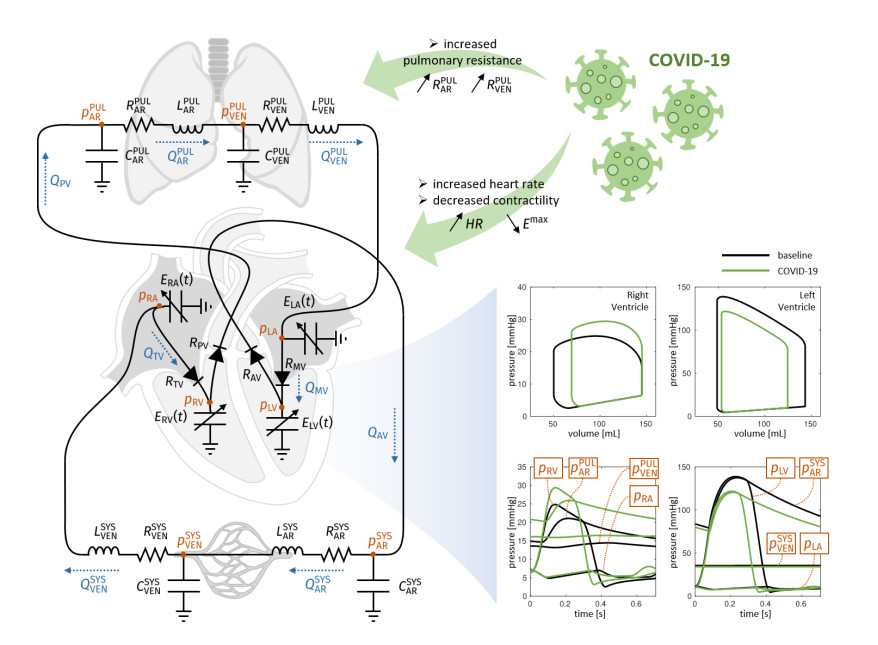
A 0D model provides a mathematical description of the function of several compartments in the cardiovascular system; their number and locations depend on the complexity of the model at hand and its level of detail. The model consists in a system of differential equations that translates physical principles such as conservation of mass and momentum. Its solution provides the values of flow rates and pressures for each compartment [10]. This system can be obtained by exploiting the electric analogy, where the current represents the blood flow, the electric potential plays the role of the pressure (and hence a voltage represents a pressure difference), the electric resistance represents the resistance to blood flow, the capacitance the vessel compliance, and the inductance the blood inertia. For a recent study on a 0D model accounting for the pulmonary circulation, see also [11]. By referring to Figure 1, our 0D model considered:
-The four heart chambers, whose mechanical behaviour was characterized by suitable model parameters. For example, for the left ventricle (LV) the unloaded volumes (i.e., volume at zero-pressure) V0LV and the time-varying elastances ELV(t) = EBLV + EALV fLV (t) were considered, where EBLV is the passive elastance (i.e., the inverse of the compliance), EALV the maximum active elastance, and fLV a function of time ranging values between 0 and 1 that accounts for the activation phases (see [12,13] for more details). Similar parameters definitions were introduced for the right ventricle (RV), left atrium (LA), and right atrium (RA). The volume of blood contained in each of the four chambers can be obtained from the solution of the following equations, that account for the inward and outward blood fluxes associated with each chamber:
In the above equations, the right-hand side terms represent the blood fluxes (mL/s) across the different cardiac valves (QMV, QAV, QTV, QPV) and through the systemic and pulmonary venous systems ($ {Q}_{VEN}^{SYS}, {Q}_{VEN}^{PUL} $). These terms will be specified later.
-The four cardiac valves modelled as diodes. More precisely, the blood flux across a valve depends on the pressure jump from the upstream to the downstream compartment:
having defined the function
where $ {R}_{min} $ and $ {R}_{max} $ are the leaflet resistances when the valve is open and closed, respectively.
-The systemic arterial circulation, characterized by the arterial resistance, capacitance and inductance RARSYS, CARSYS, LARSYS. More precisely, the blood pressure and flux associated with the systemic arterial compartment evolve according to the following laws:
Similarly, the systemic venous system is characterized by analogous parameters (i.e., RVENSYS, CVENSYS, LVENSYS), while the pulmonary circulation is characterized as above by the systemic parameters RARPUL, CARPUL, LARPUL, and by the venous ones RVENPUL, CVENPUL, LVENPUL.
The 0D model has been discretized in time by means of a variable-step, variable-order (VSVO) solver. The implementation was performed in the Matlab environment (ode15s solver). For each setting of parameters here considered, the model was run for several cycles, until a regime (periodic) solution was obtained, and only the last heartbeat was considered for the analysis.
2.2. The 3D-0D computational model
To enhance the detail of description of the 0D model presented in the previous section, one or more of its compartments can be replaced by a 3D geometrically accurate model (see e.g., [14,15] for a comprehensive review on this topic). Besides the fully 0D model for blood dynamics introduced in the previous section, in this work we considered also a 3D-0D model in which we replaced the time-varying elastance element describing the LV with a 3D multiscale electromechanical model (see Figure 4). In the 3D electromechanical model, fibers and sheets distribution were generated according to a rule-based algorithm [16]. The LV was stimulated by means of electric impulses applied at three points of the endocardial surface and the resulting action potential propagation was modelled through the monodomain equation [18] coupled with the ten Tusscher-Panfilov ionic model [17]. To describe the subcellular mechanisms of active force generation, we employed the biophysically detailed model RDQ20-MF, proposed in [19], while we employed the exponential constitutive law proposed in [20] to describe the passive behaviour of the myocardium.
We discretized the 3D ventricular electromechanical model by means of first order Finite Elements method (FEM) in space and finite differences in time [21]. To efficiently solve the coupled multiphysics 3D-0D model, we employed a segregated strategy, where electro-physiology, active forces computation, active and passive mechanics, and 0D blood dynamic model are solved in sequence, possibly with a different time step to account for the diverse temporal dynamics of each submodel. For more details on the 3D-0D electromechanical model and on the numerical methods used for its numerical approximation, we refer the interest reader to [12,13]. Such methods have been implemented in the Finite Element research library lifex (https://lifex.gitlab.io/lifex).
2.3. Variation of the model parameters
The quantities mentioned in Section 2.2 are the parameters of the model and, together with the heart rate (HR), they characterize the cardiovascular system of the individual, both in healthy and non-healthy conditions. Thus, the 0D and the 3D-0D models provide tools that are able to compute flow rate and pressure in each compartment once a suitable set of parameters is prescribed. With this aim, we identified three sources of changes in the above-mentioned parameters and corresponding reasonable value ranges:
-HR: Clinical evidence showed that an increase of HR was very common in COVID-19 patients [22]. Accordingly, we considered values of HR in the range [60,80] bpm for baseline individuals, increasing this figure up to 100 bpm for COVID patients.
-Wood number (W): It is defined as
and provides information about the pulmonary resistances. As, according to clinical evidence [23], pulmonary resistances (and thus W) increase in presence of COVID-19, we placed the value of W in the range between 1.13 (healthy) and 3.39 units. More precisely, we multiplied the baseline value RVENPUL-BLSN (see Table 1) by a factor kR in the range [1,3]:
We also assumed that RARPUL/RVENPUL = 9/10 [24]. Analogous definitions hold true for the systemic resistances;
-EAXX (where XX = LA, LV, RA, RV): Clinical evidence showed that COVID-19 may reduce blood saturation and consequently also decrease cardiomyocyte contractility. To account for this, we decreased the value of the four active elastances EAXX. Since a reliable quantitative law linking blood saturation with contractility - at the best of our knowledge - is not available in the literature, we considered the ranges of contractility variation observed in non-COVID hypoxia [25,26], by multiplying the baseline values EAXX-BLSN (see Table 1) by a percentage factor kEA in the range [50,100]%:
When the 3D-0D model is considered, the parameter EALV is not meaningful for the model, since the time-varying elastance element of the LV is replaced by the multiphysics 3D LV model. Therefore, in this case we rescaled the LV contractility, a parameter that rescales the active force generated at the microscale and that plays the role of EALV in the 3D model, by the same factor kEA. Since reduced blood saturation is not expected to affect the passive propertied of the tissue, we kept the parameters EBXX unchanged.
2.4. Setting of the clinical scenarios and description of the in silico tests
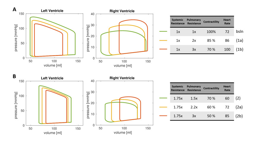
We first considered the fully 0D model in the setting reported in Table 1, corresponding to an individual in healthy conditions, henceforth denoted as baseline (bsln). With such baseline setting as a starting point, we investigated the effect of the variations mentioned above, to study a possible impact of hemodynamic changes associated with COVID-19 on the cardiac function. In particular, we considered two settings that we denoted as Test (1a) and Test (1b), respectively. In Test (1a) we decreased the contractility of the whole heart muscle to 85% of the baseline value to reflect the effects of a reduced blood saturation due to the impaired pulmonary function. Moreover, we increased HR from 72 bpm to 86 bpm and we increased the pulmonary resistance by a factor 2 (this corresponds to a Wood number W = 2.26). In Test (1b), instead, we exacerbate the three aforementioned effects, with a contractility of 70% of the baseline, a HR of 100 bpm and an increase of the pulmonary resistances by a factor 3 (Wood number 3.39). These changes from the baseline setting were suggested by clinical observations on COVID-19 patients made by the clinicians involved in this study.
We further exploited our 0D computational model by simulating the effects of COVID-19 infection for a virtual patient with mildly impaired LV cardiac function. In particular, in Test (2) we assumed that, without COVID-19, for this individual contractility was decreased to 70% of baseline, HR equal to 60 bpm, pulmonary resistance equal to 1.70 Wood (x1.5 of baseline), and systemic resistance equal to 26.25 (x1.75 of baseline) (Table 3). As in Test (1), we considered two scenarios of COVID-19 infections, with virtual impact on the cardiovascular system only, by further decreasing the heart contractility (to 60% and 50% of baseline), increasing the HR (to 72 and 85 bpm) and increasing the pulmonary resistance (to 2.54 and 3.39 Wood) for Tests (2a) and (2b), respectively. These changes from the baseline setting were suggested by observations of COVID-19 patients.
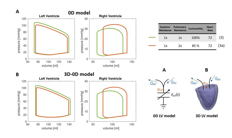
Finally, we performed a comparative analysis by means of the 0D and the 3D-0D models. We carried out a simulation with both models in a setting corresponding to an individual in healthy conditions (denoted by Test (3)), by adjusting the 0D model parameters in order to produce a LV PV loop resembling that of the 3D-0D model. Then, we perturbed both the 0D and the 3D-0D models in the same way, and we simulated the perturbed scenario – denoted as Test (3a) – with both models. Specifically, we decreased the contractility of the myocardium to 85% of the baseline value and we doubled the pulmonary resistances. Unlike the scenarios considered above, we did not alter the heart rate, because the ionic model considered in the 3D model is not designed to have a physiological response to changes of this variable [17].
3.
Results
3.1. Results of 0D numerical simulations
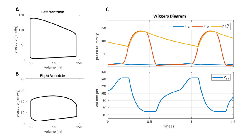
In Figure 2 we reported the outcomes predicted by the 0D model for the baseline setting. Our computational model allowed to reproduce the ventricle pressure-volume (PV) loops as well as the evolution in time of volumes and pressures with a very low computational effort nearly 2 seconds of simulation for 10 heartbeats). Table 2 reports a list of parameters of cardiac function computed by the baseline simulation. In particular, we found Cardiac Output (CO) = 6.8 L/min, Stroke Volume (SV) = 95 mL, Ejection Fraction (EF) = 66% for both LV and RV, thus the simulation reflected an overall normal cardiac function [27]. Also, LV and RV were characterized by end-diastolic volume (EDV) and end-systolic volume (ESV) within the normal ranges (LV EDV two settings, corresponding to a mild and to a more severe COVID-19 infection = 144 mL, LV ESV = 49 mL, RV EDV = 145 mL, RV ESV = 50 mL) [28,29,30].
The PV loops corresponding to the settings (1a) and (1b) are shown in Figure 3A, while Table 2 reports the corresponding cardiac measurements. These tests showed that the LV PV loops was impacted by hypoxemia, which reduced ventricular contractility. Overall, compared to baseline values, the reduced cardiac contractility provided a decrease in SV of 21% for Test (1a) and 38% for Test (1b), together with a reduction in LV EF of 11% and 25% for Test (1a) and Test (1b), respectively. This effect was partially compensated by the increase of HR, which can be considered – in hypoxic patients – as a self-regulatory mechanism aimed to preserve the CO [26]. As a matter of fact, the CO decreased 6% from baseline for Test (1a) and of 13% for Test (1b). Besides the LV function, also the RV function is significantly affected by COVID-19 related variations of the circulation model. Specifically, RV EF decreased 20% (Test (1a)) and 39% (Test (1b)), thus in percentage more than for LV. Moreover, the increased pulmonary resistance induced a remarkable growth of the RV maximal pressure (20% and 40% for Test (1a) and (1b), respectively) and the RV ESV reports a significant increase (34% and 78%).
Regarding Test (2), which represents a hypothetical individual with mildly impaired LV cardiac function, the outputs computed by the 0D model were: CO = 4.1 L/min, LV SV = 68 mL, LV EF = 50% and RV EF = 53%; moreover, we found LV EDV = 135 mL, LV ESV = 67 mL, RV EDV = 127 mL, RV ESV = 59 mL, that however were still in the normal ranges [28,29,30].
We then accounted for the change of parameters due to COVID-19 (Test (2a) and Test (2b)). The data and results are reported in Figure 3B and Table 3. The outputs of our numerical simulations highlighted that, in an individual with impaired LV cardiac function, the COVID-19 infection further worsens the cardiac functional parameters of both chambers. In particular, we found a reduction in LV EF of 14% and 30% for Test (2a) and Test (2b), respectively, in RV EF of 19% and 38%, and in CO of 5% and 10%.
3.2. Analysis of clinical scenarios
Our computational model is able to simulate possible effects of COVID-19 infection on the cardiocirculatory system, and particularly on the cardiac function. Our study sustains the clinical evidence that the infection is able to impact both the left and right hearts, by decreasing EF and CO, whose decrements are only partially compensated by the HR increase that typically is shown in COVID-19 patients. Maximum LV pressure was reduced, while maximum RV pressure was increased, albeit the latter remains within the normal range of values. Our computational model predicted that the right heart is strongly linked, from the physiopathological standpoint, to the pulmonary function. Indeed, the increased pulmonary resistance significantly affects both the RV pressure and the RV EF.
Recent data published in [31] show that lower values of RV systolic function echocardiographic parameters, although still in the normal range, are more frequent in COVID-19 patients with poor prognosis, thus suggesting that the absence of an increase in contractility in response to an increase in pulmonary resistance/pressures plays a role in the evolution of the illness. The proposed model captures this behavior. In particular, as the respiratory failure worsens, RV function is supposed to be more susceptible to impairment due to increased RV afterload and in fact we have reported a progressive decrease in RV EF volume from Test (1a) to Test (1b) for a previously healthy subject.
Since recent reports [1,2,3,4,5] suggest that CVD is a common finding in COVID-19 patients and is associated with a worse prognosis, we also simulated the cardiac function and its response to COVID-19 in a hypothetical patient with history of cardiac dysfunction. Although we predicted a reduction in LV EF when we simulate a worse COVID-19 infection, we predicted a more severe reduction in RV EF compared to the reduction in LV EF. This finding could explain the worse outcome in case of pre-existing CVD. In fact, RV dysfunction is known to be an important determinant of symptoms and a powerful marker of poor prognosis in patients with chronic heart failure [32,33].
To predict the effect of the reduced contractility, the End Systolic Pressure Volume Relationship (ESPVR) is estimated as the slope of the PV loop curve in the upper left corner [26]. The depressed inotropy corresponded to a decreased ESPVR, as reported in several experiments as a direct consequence of the reduced oxygen blood content [25,26]. As it appears in Figures 3A and 3B the proposed model highlights their effects. Moreover, the LV function experienced a reduced systolic pressure and a reduced preload, thus resulting in a significant decrease of the PVA (pressure-volume area), a further biomarker that is known to correlate with hypoxia [26,34].
From our study, we highlighted that COVID-19 infection in a patient with normal cardiac function may produce alterations that maintain biomarkers within the normal range of values. Conversely, starting from a scenario of an individual with impaired cardiac function, where however the values of biomarkers were within normal ranges [28,29,30], our simulations revealed that the COVID-19 infection could worsen the cardiac function, specifically by further reducing CO and SV below the normal values, other than severely impacting the LV and RV EFs. This computational model has been proposed to carry out results about the sensitivity of some cardiac outcomes on different parameters influenced by COVID-19 in a very rapid and reproducible way.
3.3. Comparative analysis of fully 0D and 3D-0D simulations
For the comparative analysis of fully 0D and 3D-0D simulation, we based the latter on the Zygote cardiac geometry [35], representing the average heart of a healthy Caucasian man. The computational time to perform a heartbeat was about 5 hours on 32 cores. In Figure 5 we reported the PV loops obtained for Test (3) and Test (3a) with both the fully 0D and the 3D-0D cardiovascular models. The Figure shows that the two models present a qualitatively similar response to the applied hemodynamical changes. To provide a quantitative assessment of the response of the two models, we reported in Table 4 the absolute and relative changes of some biomarkers between Test (3) and Test (3a). The results show that the two models are in great agreement quantitatively as well. The biomarker whose response differs most is LV dP/dt max, for which the 0D model predicts a 5.81% decrease, whereas the 3D-0D model predicts an 7.85% decrease. We think that the reason lies in the fact that this parameter accounts not only for the pressure-volume relationship of the ventricular chamber, but also for the characteristic time scales associated with the different physics (ionic dynamics, mechanical activation, muscle mechanics and interaction with surrounding tissues), which are much more accurately predicted by the 3D model. Nevertheless, all the other biomarkers feature a response which is always within one percentage point difference between the two models. As expected, the biomarkers associated with the RV present an even closer match.
4.
Discussion
We showed that computational models can be an effective tool to study possible effects of hemodynamic changes associated with COVID-19 on the cardiac function. In particular, this study was based on a 0D computational model, which considers compartmental flow rates and pressures. We focused on three possible consequences of COVID-19 (increased HR, decreased myocyte contractility, and increased pulmonary resistances) and on their influence on virtual patients. Our preliminary 0D model computations revealed a possible worsening of SV, CO, LV EF, RV EF, and other biomarkers for virtual clinical scenarios with both otherwise normal cardiac function and impaired cardiac function. In the latter case, these values were below normal ones even if they were within normal ranges in the case without COVID-19 effects. This provided a quantitative, although speculative, confirmation that COVID-19 could have significant consequences on the cardiac function. The comparative tests between the fully 0D and the 3D-0D models supports the appropriateness of the former to perform this type of study, which is based on analysing global quantities and outputs. In fact, the 0D model was able to predict responses to hemodynamic changes —such as those considered in this paper—in agreement with those predicted by much more sophisticated models, which provide a multiphysics and multiscale description of cardiac function. On the other hand, the use of 3D models may offer the possibility of customizing the model to specific patients using geometries acquired from medical imaging (e.g., CT or MRI), to account for spatial heterogeneities (such as the presence of scar or hypertrophic tissue), which cannot instead be included in a 0D model, and to perform 3D analysis of computed maps, localising possible damaged behaviours.
Several limitations affected this preliminary work. First, we notice that our 0D model is rather simple in comparison to other models reported so far for the study of the cardiac function (see, e.g., [36,37,38,39]), although it is capable to recover significant and clinically meaningful results such as PV-loops. Moreover, our model did not account for the integration with the respiratory system, as done elsewhere [38,39]. A model that directly accounts for the variation of blood saturation due to COVID-19 is currently under development: we expect that it could lead our study to an improved degree of novelty. Also, we neglected the effect of pressure variations due to respiration on the rib cage, hence on the cardiocirculatory system. Albeit we deem this assumption to have a very limited impact on the outcomes of the current study, we plan to improve our 0D model for further investigations of this topic.
Second, we accounted for possible changes induced by COVID-19 (pulmonary resistances, heart rate, contractility), which are however not specific of COVID-19 and could occur also in other diseases that lead to heart failure [36,37,38,39]. For example, other studies investigated by means of 0D models possible effects in patients affected by Chronic Obstructive Pulmonary Disease (COPD) [40], obtaining similar results to ours in terms of decreased cardiac function. How COVID-19 does influence the cardiovascular system and the heart function in a specific way that characterizes this virus is still far from being known at the patho-physiological level. For example, interactions with diseases that damage also, e.g., the respiratory system, the liver, the kidney, the brain should characterize this multiorgan disease. However, due to the lack of precise information on such mechanisms, we have limited ourselves to account here only for the indisputable sources of change.
Also, we observe that the pathophysiology of COVID-19 involves several systems, such as the neurohormonal system (e.g., with production of cytokines), the systemic circulation, and the coronary perfusion. Moreover, it could involve remodelling and compensatory mechanisms, such as those related to myocardial oxygen consumption that can be well preserved even under severe hypoxia. Similarly, factors such as gender and age have not been included in the model yet. However, the interactions among all these processes have not yet been fully understood. Moreover, the mathematical description of their coupling is still far to be ready for applications. For these reasons, such interactions were not included in this work. However, we included some effects of the insult provided by the virus on the neuronal system, such as the increment of heart rate and of the pulmonary resistances. We remark that the aim of this work was not to develop an omni-comprehensive model, but rather to build a cardiovascular model focused on the cardiopulmonary interactions only, that is those occurring among the heart, vasculature, and lungs. We notice also that COVID-19 effects on the organism may differ along the progression of the disease [41], an assessment that we have not included in our model, which was rather focused on the final effect on the cardiac function.
Another limitation is that only virtual (healthy or not) individuals were considered to study the possible effect of COVID-19 on the cardiac function. In particular, we selected representative parameter values to run our numerical simulations. This represents a current limitation as the parameters may considerably differ among patients, in particular as a response to COVID-19 infection. The collection of data and measures regarding COVID-19 patients could allow us in the next future to build models that are patient-specific (by suitably calibrating the parameters) and to provide answers to specific clinical questions. In the meantime, we believe that the study on virtual patients is fundamental as a preliminary step in view of assessing the potential effectiveness of our approach for clinical scenarios.
In order to partially overcome to some of the previous limitations, a more detailed study for predicting pointwise quantities of interest in the heart could be carried out by means of a 3D-0D model, where the heart (or a part of it) is simulated by means of a 3D electromechanical model; in this model, the computational geometry of the heart can be personalized starting from clinical images (CT or MRI) acquired from a specific patient. The 3D-0D numerical tests shown in this paper support the feasibility of this approach. Another improvement could be obtained by coupling the 0D (or even 3D-0D) model with the cardiac perfusion in order to quantify the amount of blood flow reaching the myocardium [42] and with a model for oxygen–hemoglobin association-dissociation to quantify the oxygen supply to the heart.
5.
Conclusions
Despite the aforementioned limitations of our study, we believe that this paper represents a first, necessary step towards a more comprehensive model. Indeed, the goal of this study was to propose a model to quantitatively analyze the interactions between the heart and the lungs in COVID-19 patients. In particular, the model allowed us to include the effect of comorbidities related to the cardiovascular system, but not others of different nature. However, this study can provide the basis for further developments in which other organ systems and other interactions, once understood from the clinical experience, are included in the model.
This study paves the way for a better understanding of the interplay between COVID-19 and cardiovascular dysfunction and diseases. As a matter of fact, even if cardiac involvement is a prominent feature in COVID-19 and is associated with a worse prognosis, the response of the cardiovascular system to COVID-19 infection has not been well studied yet [1,2,3,4,5]. This study lends support to the impact of COVID-19 on the cardiac function in patients with or without cardiovascular disease. Our computational approach could be an effective tool to study the patient specific effect of COVID-19 on the cardiac function.
Acknowledgments
L. Dede', A. Quarteroni, C. Vergara and P. Zunino have been supported by the Italian research project MIUR PRIN17 2017AXL54F "Modeling the heart across the scales: from cardiac cells to the whole organ". F. Regazzoni has been supported by the Italian research project MIUR PRIN17 2017KL4EF3 "Mathematics of active materials: From mechanobiology to smart devices".
Conflict of interest
The authors declare that they have no conflict of interest with industries or other.


 DownLoad: