On generalized active contour model in the anisotropic BV space and its application to satellite remote sensing of agricultural territory

Ciro D'Apice; Peter Kogut; Rosanna Manzo; Ciro D'Apice; Peter Kogut; Rosanna Manzo

doi:10.3934/nhm.2025008

Networks and Heterogeneous Media

2025, Volume 20, Issue 1: 113-142. doi: 10.3934/nhm.2025008

Previous Article Next Article

Research article

On generalized active contour model in the anisotropic BV space and its application to satellite remote sensing of agricultural territory

1.
Dipartimento di Scienze Aziendali-Management and Information Systems, University of Salerno, Via Giovanni Paolo Ⅱ, 132, Fisciano (SA), 84084, Italy
2.
Department of Differential Equations, Oles Honchar Dnipro National University, Gagarin av., 72, 49010 Dnipro, Ukraine
3.
EOS Data Analytics Ukraine, Gagarin av., 103a, Dnipro, Ukraine
4.
Dipartimento di Scienze Politiche e della Comunicazione, University of Salerno, Via Giovanni Paolo Ⅱ, 132, Fisciano (SA), 84084, Italy

Received: 17 November 2024 Revised: 01 February 2025 Accepted: 07 February 2025 Published: 13 February 2025

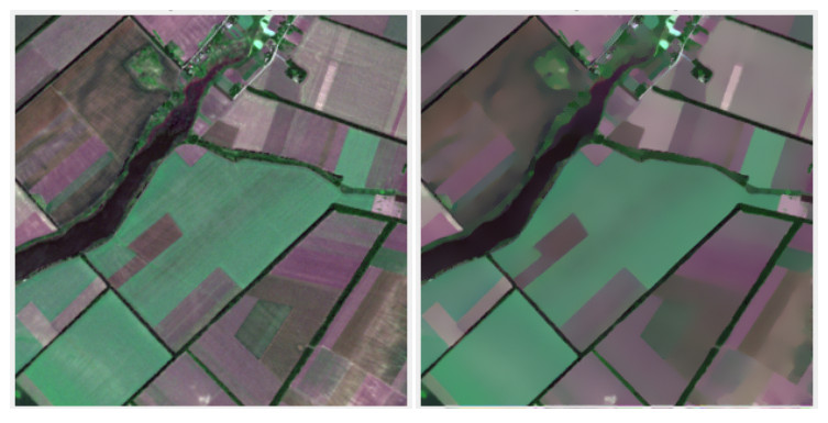
Mostly motivated by the crop field classification problem and the automated computational methodology for extracting agricultural crop fields from satellite data, we proposed in a bounded variation (BV) space a new approach to the piecewise smooth approximation of the slope-based vegetation indices and the closely related crop field segmentation problem of multi-band satellite images.
- optimal segmentation problem,
- piecewise smooth approximation,
- existence result,
- optimality conditionso,
- level set method,
- partial differential equation,
- active contour model
Citation: Ciro D'Apice, Peter Kogut, Rosanna Manzo. On generalized active contour model in the anisotropic BV space and its application to satellite remote sensing of agricultural territory[J]. Networks and Heterogeneous Media, 2025, 20(1): 113-142. doi: 10.3934/nhm.2025008

Related Papers:

Abstract

Mostly motivated by the crop field classification problem and the automated computational methodology for extracting agricultural crop fields from satellite data, we proposed in a bounded variation (BV) space a new approach to the piecewise smooth approximation of the slope-based vegetation indices and the closely related crop field segmentation problem of multi-band satellite images.

References

[1]	R. Boesch, Z. Wang, Segmentation optimization for aerial images with spacial constraints, in The International Archives of the Photogrammetry, Remote Sensing and Spatial Information Sciences, 37 (2008), 285–289.
[2]	Y. Chen, Q. Chen, C. Jing, Multi-resolution segmentation parameters optimization and evaluation for VHR remote sensing image based on meanNSQI and discrepancy measure, J. Spat. Sci., 66 (2019), 253–278. https://doi.org/10.1080/14498596.2019.1615011 doi: 10.1080/14498596.2019.1615011
[3]	P. Xiao, X. Zhang, H. Zhang, R. Hu, X. Feng, Multiscale optimized segmentation of urban green cover in high resolution remote sensing image, Remote Sens., 10 (2018), 1813. https://doi.org/10.3390/rs10111813 doi: 10.3390/rs10111813
[4]	J. Xue, B. Su, Significant remote sensing Vegetation Indices: A review of developments and applications, J. Sensors, 2017 (2017), 1353691. https://doi.org/10.1155/2017/1353691 doi: 10.1155/2017/1353691
[5]	D. Mumford, J. Shah, Optimal approximation by piecewise smooth functions and associated variational problems, Commun. Pure. Appl. Math., 42 (1989), 577–685. https://doi.org/10.1002/cpa.3160420503 doi: 10.1002/cpa.3160420503
[6]	L. Alvarez, P. L. Lions, J. M. Morel, Image selective smoothing and edge detection by nonlinear diffusion. Ⅱ, SIAM J. Numer. Anal., 29 (1992), 845–866. https://doi.org/10.1137/0729052 doi: 10.1137/0729052
[7]	L. Alvarez, F. Guichard, P. L. Lions, J. M. Morel, Axioms and fundamental equations of image processing, Arch. Ration. Mech. Anal., 123 (1993), 199–257. https://doi.org/10.1007/BF00375127 doi: 10.1007/BF00375127
[8]	F. Catté, T. Coll, P. L. Lions, J. M. Morel, Image selective smoothing and edge detection by nonlinear diffusion. Ⅰ, SIAM J. Numer. Anal., 29 (1992), 182–193. https://doi.org/10.1137/0729012 doi: 10.1137/0729012
[9]	V. Caselles, R. Kimmel, G. Sapiro, Geodesic active contours, Int. J. Comput. Vision, 22 (1997), 61–79. https://doi.org/10.1023/A:1007979827043 doi: 10.1023/A:1007979827043
[10]	T. Chan, L. Vese, Active contours without edges, IEEE Trans. Image Process., 10 (2001), 266–277. https://doi.org/10.1109/83.902291 doi: 10.1109/83.902291
[11]	D. J. Mulla, Twenty five years of remote sensing in precision agriculture: Key advances and remaining knowledge gaps, Biosyst. Eng., 114 (2013), 358–371. https://doi.org/10.1016/j.biosystemseng.2012.08.009 doi: 10.1016/j.biosystemseng.2012.08.009
[12]	B. Han, Y. Wu, Active contour model for inhomogeneous image segmentation based on Jeffreys divergence, Pattern Recognit., 107 (2020), 107520. http://dx.doi.org/10.1016/j.patcog.2020.107520 doi: 10.1016/j.patcog.2020.107520
[13]	H. Jeffreys, An invariant form for the prior probability in estimation problems, Proc. R. Soc. Lond., Ser. A, Math. Phys. Sci., 186 (1946), 453–461. https://doi.org/10.1098/rspa.1946.0056 doi: 10.1098/rspa.1946.0056
[14]	C. Yang, G. Weng, Y. Chen, Active contour model based on local Kullback–Leibler divergence for fast image segmentation, Eng. Appl. Artif. Intell., 123 (2023), 106472. https://doi.org/10.1016/j.engappai.2023.106472 doi: 10.1016/j.engappai.2023.106472
[15]	C. Samson, L. Blanc-Féraud, G. Aubert, J. Zerubia, Multiphase Evolution and Variational Image Classification, INRIA Sophia Antipolis, 1999.
[16]	H. Attouch, G. Buttazzo, G. Michaille, Variational Analysis in Sobolev and $BV$ Spaces: Applications to PDEs and Optimization, Philadelphia: SIAM, 2006.
[17]	L. C. Evans, Weak convergence methods for nonlinear partial differential equations, Washington, DC: American Mathematical Society, 1990.
[18]	L. Ambrosio, N. Fusco, D. Pallara, Functions of Bounded Variation and Free Discontinuity Problems, New York: Oxford University Press, 2000.
[19]	E. Giusti, Minimal Surfaces and Functions of Bounded Variation, Boston: Birkhäuser, 1984. https://doi.org/10.1007/978-1-4684-9486-0
[20]	L. C. Evans, R. E. Gariepy, Measure Theory and Fine Properties of Functions, New York: Routledge, 1992. https://doi.org/10.1201/9780203747940
[21]	R. Caccioppoli, Misura e integrazione sugli insiemi dimensionalmente orientali Ⅰ.Ⅱ, Atti Accad. Naz. Lincei. Rend. Cl. Sci. Fis. Mat. Nat., 12 (1952), 3–11.
[22]	M. Grasmair, A Coarea Formula for Anisotropic Total Variation Regularisation, Universität Wien, 2010.
[23]	L. Rotem, The anisotropic total variation and surface area measures, In: Geometric Aspects of Functional Analysis, Cham: Springer, 2327 (2023), 297–312. https://doi.org/10.1007/978-3-031-26300-2_11
[24]	L. Bungert, D. A. Coomes, M. J. Ehrhardt, J. Rasch, R. Reisenhofer, R. C. B. Schönlieb, Blind image fusion for hyperspectral imaging with the directional total variation, Inverse Probl., 34 (2018), 044003. https://doi.org/10.1088/1361-6420/aaaf63 doi: 10.1088/1361-6420/aaaf63
[25]	L. Bar, T. F. Chan, G. Chung, M. Jung, N. Kiryati, R. Mohieddine, N. Socheen, L. A. Vese, Mumford and Shah model and its applications to image segmentation and image restoration, In: Handbook of Mathematical Methods in Imaging, New York: Springer, 2011, 1097–1157. https://doi.org/10.1007/978-0-387-92920-0_25
[26]	T. Chan, L. Vese, A level set algorithm for minimizing the Mumford-Shah functional in image processing, in Proceedings IEEE Workshop on Variational and Level Set Methods in Computer Vision, 2001,161–168. https://doi.org/10.1109/VLSM.2001.938895
[27]	G. Dal Maso, An Introduction to $\Gamma$-Convergence, Boston: Birkhäuser Verlag, 1993. https://doi.org/10.1007/978-1-4612-0327-8
[28]	P. I. Kogut, O. P. Kupenko, Approximation Methods in Optimization of Nonlinear Systems, Berlin, Boston: De Gruyter, 2019. https://doi.org/10.1515/9783110668520
[29]	P. I. Kogut, G. Leugering, Optimal control problems for partial differential equations on reticulated domains. Approximation and Asymptotic Analysis, Boston: Birkhäuser Verlag, 2011. https://doi.org/10.1007/978-0-8176-8149-4
[30]	C. D'Apice, P. I. Kogut, O. Kupenko, R. Manzo, On a variational problem with a nonstandard growth functional and its applications to image processing, J. Math. Imaging Vision, 65 (2023), 472–491. https://doi.org/10.1007/s10851-022-01131-w doi: 10.1007/s10851-022-01131-w

Reader Comments

Your name:*

Email:*
© 2025 the Author(s), licensee AIMS Press. This is an open access article distributed under the terms of the Creative Commons Attribution License (http://creativecommons.org/licenses/by/4.0)