High-order schemes for the fractional coupled nonlinear Schrödinger equation

Fengli Yin; Dongliang Xu; Wenjie Yang; Fengli Yin; Dongliang Xu; Wenjie Yang

doi:10.3934/nhm.2023063

Networks and Heterogeneous Media

2023, Volume 18, Issue 4: 1434-1453. doi: 10.3934/nhm.2023063

Previous Article Next Article

Research article

High-order schemes for the fractional coupled nonlinear Schrödinger equation

1.
Zhoukou Normal University, Zhoukou 466000, China
2.
Nanjing University of Finance and Economics Hongshan College, Nanjing 210023, China
3.
School of Science, Xuchang University, Xuchang 461000, China

Received: 14 March 2023 Revised: 19 May 2023 Accepted: 31 May 2023 Published: 15 June 2023

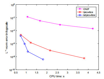
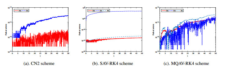
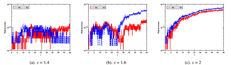
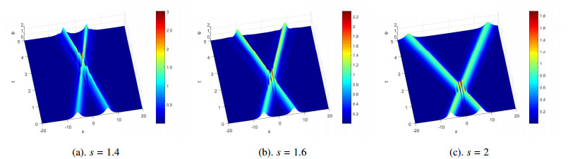
This paper considers the fractional coupled nonlinear Schrödinger equation with high degree polynomials in the energy functional that cannot be handled by using the quadratic auxiliary variable method. To this end, we develop the multiple quadratic auxiliary variable approach and then construct a family of structure-preserving schemes with the help of the symplectic Runge-Kutta method for solving the equation. The given schemes have high accuracy in time and can both inherit the mass and Hamiltonian energy of the system. Ample numerical results are given to confirm the accuracy and conservation of the developed schemes at last.
- multiple quadratic auxiliary variable,
- fractional coupled Schrödinger equation,
- conservative schemes,
- high-accuracy,
- numerical stability
Citation: Fengli Yin, Dongliang Xu, Wenjie Yang. High-order schemes for the fractional coupled nonlinear Schrödinger equation[J]. Networks and Heterogeneous Media, 2023, 18(4): 1434-1453. doi: 10.3934/nhm.2023063

Related Papers:

Abstract

This paper considers the fractional coupled nonlinear Schrödinger equation with high degree polynomials in the energy functional that cannot be handled by using the quadratic auxiliary variable method. To this end, we develop the multiple quadratic auxiliary variable approach and then construct a family of structure-preserving schemes with the help of the symplectic Runge-Kutta method for solving the equation. The given schemes have high accuracy in time and can both inherit the mass and Hamiltonian energy of the system. Ample numerical results are given to confirm the accuracy and conservation of the developed schemes at last.

References

[1]	L. Brugnano, C. Zhang, D. Li, A class of energy-conserving Hamiltonian boundary value methods for nonlinear Schrödinger equation with wave operator, Commun. Nonlinear Sci. Numer. Simul., 60 (2018), 33–49.
[2]	Y. Chen, Y. Gong, C. Wang, Q. Hong, A new class of high-order energy-preserving schemes for the Korteweg-de Vries equation based on the quadratic auxiliary variable (QAV) approach, arXiv: 2108.12097, [Preprint], (2021) [cited 2023 June 15].
[3]	Q. Cheng, The generalized scalar auxiliary variable approach (G-SAV) for gradient flows, arXiv: 2002.00236, [Preprint], (2020) [cited 2023 June 15]. Available from: https://doi.org/10.48550/arXiv.2002.00236
[4]	J. Cui, Y. Wang, C. Jiang, Arbitrarily high-order structure-preserving schemes for the Grossc-Pitaevskii equation with angular momentum rotation, Comput. Phys. Commun., 261 (2021), 107767.
[5]	J. Cui, Z. Xu, Y. Wang, C. Jiang, Mass-and energy-preserving exponential Runge-Kutta methods for the nonlinear Schrödinger equation, Appl. Math. Lett., 112 (2020), 106770.
[6]	S. Duo, Y. Zhang, Mass-conservative Fourier spectral methods for solving the fractional nonlinear Schrödinger equation, Comput. Math. Appl., 71 (2016), 2257–2271. https://doi.org/10.1016/j.camwa.2015.12.042 doi: 10.1016/j.camwa.2015.12.042
[7]	Y. Fu, W. Cai, Y. Wang, A linearly implicit structure-preserving scheme for the fractional sine-Gordon equation based on the IEQ approach, Appl. Numer. Math., 160 (2021), 368–385. https://doi.org/10.1016/j.apnum.2020.10.009 doi: 10.1016/j.apnum.2020.10.009
[8]	Y. Fu, D. Hu, Y. Wang, High-order structure-preserving algorithms for the multi-dimensional fractional nonlinear Schrödinger equation based on the SAV approach, Math. Comput. Simul., 185 (2021), 238–255.
[9]	Y. Gong, J. Zhao, X. Yang, Q. Wang, Fully discrete second-order linear schemes for hydrodynamic phase field models of binary viscous fluid flows with variable densities, SIAM J. Sci. Comput., 40 (2018), B138–B167.
[10]	X. Gu, Y. Zhao, X. Zhao, B. Carpentieri, Y. Huang, A note on parallel preconditioning for the all-at-once solution of riesz fractional diffusion equations, Numer. Math. Theor. Meth. Appl., 14 (2021), 893–919.
[11]	B. Guo, Z. Huo, Global well-posedness for the fractional nonlinear Schrödinger equation, Commun. Partial Differ. Equ., 36 (2010), 247–255. https://doi.org/10.1080/03605302.2010.503769 doi: 10.1080/03605302.2010.503769
[12]	E. Hairer, C. Lubich, G. Wanner, Solving Geometric Numerical Integration: Structure-Preserving Algorithms, Berlin: Springer, 2006.
[13]	J. Hu, J. Xin, H. Lu, The global solution for a class of systems of fractional nonlinear Schrödinger equations with periodic boundary condition, Comput. Math. Appl., 62 (2011), 1510–1521. https://doi.org/10.1016/j.camwa.2011.05.039 doi: 10.1016/j.camwa.2011.05.039
[14]	C. Jiang, Y. Wang, Y. Gong, Explicit high-order energy-preserving methods for general Hamiltonian partial differential equations, J. Comput. Appl. Math., 388 (2020), 113298. https://doi.org/10.1016/j.cam.2020.113298 doi: 10.1016/j.cam.2020.113298
[15]	A. Khaliq, X. Liang, K. M. Furati, A fourth-order implicit-explicit scheme for the space fractional nonlinear Schrödinger equations, Numer. Algorithms., 75 (2017), 147–172. https://doi.org/10.1007/s11075-016-0200-1 doi: 10.1007/s11075-016-0200-1
[16]	N. Laskin, Fractional quantum mechanics, Phys. Rev. E., 62 (2000), 3135–3145. https://doi.org/10.1103/PhysRevE.62.3135 doi: 10.1103/PhysRevE.62.3135
[17]	N. Laskin, Fractional quantum mechanics and Lévy path integrals, Phys. Lett. A., 268 (2000), 298–305. https://doi.org/10.1016/S0375-9601(00)00201-2 doi: 10.1016/S0375-9601(00)00201-2
[18]	N. Laskin, Fractional Schrödinger equation, Phys. Rev. E., 66 (2002), 056108. https://doi.org/10.1103/PhysRevE.66.056108 doi: 10.1103/PhysRevE.66.056108
[19]	D. Li, W. Sun, Linearly Implicit and High-Order Energy-Conserving Schemes for Nonlinear Wave Equations, J. Sci. Comput., 83 (2020), 1–17. https://doi.org/10.1007/s10915-020-01189-x doi: 10.1007/s10915-020-01189-x
[20]	G. Akrivis, D. Li, Structure-preserving Gauss methods for the nonlinear Schrödingerequation, Calcolo, 58 (2021), 1–25.
[21]	H. Li, Y. Wang, M. Qin, A sixth order averaged vector field method, J. Comput. Math., 34 (2016), 479–498. https://doi.org/10.4208/jcm.1601-m2015-0265 doi: 10.4208/jcm.1601-m2015-0265
[22]	M. Li, X. Gu, C. Huang, M. Fei, G. Zhang, A fast linearized conservative finite element method for the strongly coupled nonlinear fractional Schrödinger equations, J. Comput. Phys., 358 (2018), 256–282. https://doi.org/10.1016/j.jcp.2017.12.044 doi: 10.1016/j.jcp.2017.12.044
[23]	M. Li, C. Huang, P. Wang, Galerkin finite element method for nonlinear fractional Schrödinger equations, Numer. Algorithms., 74 (2017), 499–525. https://doi.org/10.1007/s11075-016-0160-5 doi: 10.1007/s11075-016-0160-5
[24]	M. Li, C. Huang, Z. Zhang, Unconditional error analysis of Galerkin FEMs for nonlinear fractional Schrödinger equation, Appl. Anal., 97 (2018), 295–315. https://doi.org/10.1080/00036811.2016.1262947 doi: 10.1080/00036811.2016.1262947
[25]	Z. Liu, X. Li, The exponential scalar auxiliary variable (E-SAV) approach for phase field models and its explicit computing, SIAM J. Sci. Comput., 42 (2019), B630–B655. https://doi.org/10.1137/19M1305914 doi: 10.1137/19M1305914
[26]	M. Ran, C. Zhang, A conservative difference scheme for solving the strongly coupled nonlinear fractional Schrödinger equations, Commun. Nonlinear. Sci. Numer.Simul., 41 (2016), 64–83. https://doi.org/10.1016/j.cnsns.2016.04.026 doi: 10.1016/j.cnsns.2016.04.026
[27]	J. Shen, J. Xu, J. Yang, A new class of efficient and robust energy stable schemes for gradient flows, SIAM Rev., 61 (2019), 474–506. https://doi.org/10.1137/17M1150153 doi: 10.1137/17M1150153
[28]	J. Sun, X. Gu, Z. Ma, Numerical study of the soliton waves of the coupled nonlinear Schrödinger system, Phys. D, 196 (2004), 311–328. https://doi.org/10.1016/j.physd.2004.05.010 doi: 10.1016/j.physd.2004.05.010
[29]	D. Wang, A. Xiao, W. Yang, Crank–Nicolson difference scheme for the coupled nonlinear Schrödinger equations with the Riesz space fractional derivative. J. Comput. Phys., 242 (2013), 670–681.
[30]	D. Wang, A. Xiao, W. Yang, A linearly implicit conservative difference scheme for the space fractional coupled nonlinear Schrödinger equations, J. Comput. Phys., 272 (2014), 644–655. https://doi.org/10.1016/j.jcp.2014.04.047 doi: 10.1016/j.jcp.2014.04.047
[31]	D. Wang, A. Xiao, W. Yang, Maximum-norm error analysis of a difference scheme for the space fractional CNLS, Appl. Math. Comput., 257 (2015), 241–251. https://doi.org/10.1016/j.amc.2014.11.026 doi: 10.1016/j.amc.2014.11.026
[32]	P. Wang, C. Huang, A conservative linearized difference scheme for the nonlinear fractional Schrödinger equation, Numer. Algorithms., 69 (2015), 625–641. https://doi.org/10.1007/s11075-014-9917-x doi: 10.1007/s11075-014-9917-x
[33]	P. Wang, C. Huang, Structure-preserving numerical methods for the fractional Schrödinger equation, Appl. Numer. Math., 129 (2018), 137–158. https://doi.org/10.1016/j.apnum.2018.03.008 doi: 10.1016/j.apnum.2018.03.008
[34]	Y. Wang, L. Mei, Q. Li, L. Bu, Split-step spectral Galerkin method for the two-dimensional nonlinear space-fractional Schrödinger equation, Appl. Numer. Math., 136 (2019), 257–278. https://doi.org/10.1016/j.apnum.2018.10.012 doi: 10.1016/j.apnum.2018.10.012
[35]	A. Xiao, J. Wang, Symplectic scheme for the Schrödinger equation with fractional laplacian, Appl. Numer. Math., 146 (2019), 469–487. https://doi.org/10.1016/j.apnum.2019.08.002 doi: 10.1016/j.apnum.2019.08.002
[36]	X. Yang, J. Zhao, Q. Wang, Linear, first and second-order, unconditionally energy stable numerical schemes for the phase field model of homopolymer blends, J. Comput. Phys., 327 (2016), 294–316. https://doi.org/10.1016/j.jcp.2016.09.029 doi: 10.1016/j.jcp.2016.09.029
[37]	X. Zhao, Z. Sun, Z. Hao, A fourth-order compact ADI scheme for two-dimensional nonlinear space fractional Schrödinger equation, SIAM. J. Comput., 36 (2014), A2865–A2886. https://doi.org/10.1137/140961560 doi: 10.1137/140961560

Reader Comments

Your name:*

Email:*
© 2023 the Author(s), licensee AIMS Press. This is an open access article distributed under the terms of the Creative Commons Attribution License (http://creativecommons.org/licenses/by/4.0)