Loading [MathJax]/jax/element/mml/optable/BasicLatin.js
 

A new DG method for a pure–stress formulation of the Brinkman problem with strong symmetry

  • Received: 01 April 2022 Revised: 01 August 2022 Published: 25 August 2022
  • 65N30, 65M12, 65M15, 74H15

  • A strongly symmetric stress approximation is proposed for the Brinkman equations with mixed boundary conditions. The resulting formulation solves for the Cauchy stress using a symmetric interior penalty discontinuous Galerkin method. Pressure and velocity are readily post-processed from stress, and a second post-process is shown to produce exactly divergence-free discrete velocities. We demonstrate the stability of the method with respect to a DG-energy norm and obtain error estimates that are explicit with respect to the coefficients of the problem. We derive optimal rates of convergence for the stress and for the post-processed variables. Moreover, under appropriate assumptions on the mesh, we prove optimal L2-error estimates for the stress. Finally, we provide numerical examples in 2D and 3D.

    Citation: Salim Meddahi, Ricardo Ruiz-Baier. A new DG method for a pure–stress formulation of the Brinkman problem with strong symmetry[J]. Networks and Heterogeneous Media, 2022, 17(6): 893-916. doi: 10.3934/nhm.2022031

    Related Papers:

    [1] Patrick Henning, Mario Ohlberger . The heterogeneous multiscale finite element method for advection-diffusion problems with rapidly oscillating coefficients and large expected drift. Networks and Heterogeneous Media, 2010, 5(4): 711-744. doi: 10.3934/nhm.2010.5.711
    [2] Verónica Anaya, Mostafa Bendahmane, David Mora, Ricardo Ruiz Baier . On a vorticity-based formulation for reaction-diffusion-Brinkman systems. Networks and Heterogeneous Media, 2018, 13(1): 69-94. doi: 10.3934/nhm.2018004
    [3] Javier A. Almonacid, Gabriel N. Gatica, Ricardo Oyarzúa, Ricardo Ruiz-Baier . A new mixed finite element method for the n-dimensional Boussinesq problem with temperature-dependent viscosity. Networks and Heterogeneous Media, 2020, 15(2): 215-245. doi: 10.3934/nhm.2020010
    [4] Lan Zhu, Li Xu, Jun-Hui Yin, Shu-Cheng Huang, Bin Li . A discontinuous Galerkin Method based on POD model reduction for Euler equation. Networks and Heterogeneous Media, 2024, 19(1): 86-105. doi: 10.3934/nhm.2024004
    [5] Yue Tai, Xiuli Wang, Weishi Yin, Pinchao Meng . Weak Galerkin method for the Navier-Stokes equation with nonlinear damping term. Networks and Heterogeneous Media, 2024, 19(2): 475-499. doi: 10.3934/nhm.2024021
    [6] Zhangxin Chen . On the control volume finite element methods and their applications to multiphase flow. Networks and Heterogeneous Media, 2006, 1(4): 689-706. doi: 10.3934/nhm.2006.1.689
    [7] Lifang Pei, Man Zhang, Meng Li . A novel error analysis of nonconforming finite element for the clamped Kirchhoff plate with elastic unilateral obstacle. Networks and Heterogeneous Media, 2023, 18(3): 1178-1189. doi: 10.3934/nhm.2023050
    [8] Xiongfa Mai, Ciwen Zhu, Libin Liu . An adaptive grid method for a singularly perturbed convection-diffusion equation with a discontinuous convection coefficient. Networks and Heterogeneous Media, 2023, 18(4): 1528-1538. doi: 10.3934/nhm.2023067
    [9] Huanhuan Li, Meiling Ding, Xianbing Luo, Shuwen Xiang . Convergence analysis of finite element approximations for a nonlinear second order hyperbolic optimal control problems. Networks and Heterogeneous Media, 2024, 19(2): 842-866. doi: 10.3934/nhm.2024038
    [10] JinJun Yong, Changlun Ye, Xianbing Luo . A fully discrete HDG ensemble Monte Carlo algorithm for a heat equation under uncertainty. Networks and Heterogeneous Media, 2025, 20(1): 65-88. doi: 10.3934/nhm.2025005
  • A strongly symmetric stress approximation is proposed for the Brinkman equations with mixed boundary conditions. The resulting formulation solves for the Cauchy stress using a symmetric interior penalty discontinuous Galerkin method. Pressure and velocity are readily post-processed from stress, and a second post-process is shown to produce exactly divergence-free discrete velocities. We demonstrate the stability of the method with respect to a DG-energy norm and obtain error estimates that are explicit with respect to the coefficients of the problem. We derive optimal rates of convergence for the stress and for the post-processed variables. Moreover, under appropriate assumptions on the mesh, we prove optimal L2-error estimates for the stress. Finally, we provide numerical examples in 2D and 3D.


    Scope and related work. Brinkman equations constitute one of the simplest homogenized models for viscous fluid flow in highly heterogeneous porous media. The analysis of the underlying PDE system exhibits challenges due to the presence of two parameters: viscosity and permeability. Likewise, the design and analysis of numerical methods that maintain robustness with respect to the very relevant cases of low effective viscosity (Darcy-like regime) vs very large permeability (Stokes-like regime), is still an issue of high interest.

    For classical velocity–pressure formulations, a number of contributions are available to deal with the inf-sup compatibility of velocity and pressure spaces irrespective of the regime (Darcy-like or Stokes-like). See, e.g., [17,18,20,21,23]. On the other hand, mixed finite element formulations for Brinkman equations (that is, using other fields apart from the classical velocity–pressure pair) include pseudostress–based methods [14,19] (see also VEM counterparts in [8,15], and [26] for the DG case with strong imposition of pseudostress symmetry, closer to the present contribution), vorticity–velocity–pressure schemes in augmented and non-augmented form [3-6,28]. There, the analysis of continuous and discrete problems depends either on the Babuška–Brezzi theory, or on a generalized inf-sup argument.

    The method advanced in this paper is based on a pure–stress formulation, obtained from taking the deviatoric part of the stress and eliminating pressure, and using the momentum equation to write velocity as a function of the external and internal forces (forcing plus the divergence of the Cauchy stress). We consider the case of mixed boundary conditions, and use a symmetric interior penalty DG discretization. The space for discrete stresses incorporates symmetry strongly, as in [26] (see also [29] for elasticity and [25] for viscoelasticity). At the discrete level, the velocity and the pressure are easily recovered in terms of the discrete Cauchy stress through post-processing. While the pressure post-processing is derivative-free, the usual post-process of velocity through the momentum balance entails taking the discrete divergence of the approximate stress. We also propose a more involved reconstruction, starting from the initial post-processed velocity and solving an additional problem in mixed form using H(div)-conforming approximations. The newly computed velocity is exactly divergence-free and we prove that it enjoys the same convergence order as the stress approximation.

    Other advantages of the present formulation include the physically accurate imposition of outflow boundary conditions fixing the normal traces of the full Cauchy stress (which is not straightforward to incorporate with vorticity- or pseudostress-based methods), having symmetric and positive definite linear systems after discretization, and straightforwardly handling heterogeneous and anisotropic permeability distributions. In this regard, the analysis of the formulation uses a DG-energy norm chosen in such a way that the error estimates are independent of the jumps of the permeability. This implies a similar property concerning the estimates for the velocity approximation. However, for the pressure we can only achieve stability and optimal rates of convergence in terms of the mesh parameter.

    Outline. The contents of the paper have been laid out in the following manner. The remainder of this Section lists useful notation regarding tensors, and it recalls the definition of Sobolev spaces, inner products, and integration by parts. In Section 2 we state the Brinkman problem, specify assumptions on the model coefficients, and derive a weak formulation written only in terms of stress. Section 3 gathers the preliminary concepts needed for the construction and analysis of the discrete problem. Here we include mesh properties, recall useful trace and inverse inequalities, define suitable projectors, and establish approximation properties in conveniently chosen norms. The definition of the stress-based DG method and the proof its consistency and optimal convergence in the stress variable is presented in Section 4. The velocity and pressure post-processing, together with the corresponding error estimates, are given in Section 5. Next, in Section 6 we derive optimal error bounds for the stress in the L2-norm, and Section 7 contains a collection of numerical examples that confirm experimentally the convergence of the method, and also showcase its application into typical flow problems in 2D and 3D.

    Notational preliminaries. We denote the space of real matrices of order d×d by M and let S:={τM; τ=τt} be the subspace of symmetric matrices, where τt:=(τji) stands for the transpose of τ=(τij). The component-wise inner product of two matrices σ,τM is defined by σ:τ:=i,jσijτij. We also introduce the deviatoric part τD:=τ1d(trτ)I of a tensor τ, where trτ:=di=1τii and I stands here for the identity in M.

    Let Ω be a polyhedral Lipschitz bounded domain of Rd (d=2,3), with boundary Ω. Along this paper we convene to apply all differential operators row-wise. Hence, given a tensorial function σ:ΩM and a vector field u:ΩRd, we set the divergence divσ:ΩRd, the gradient u:ΩM, and the linearized strain tensor ε(u):ΩS as

    (divσ)i:=jjσij,(u)ij:=jui,andε(u):=12[u+(u)t].

    For sR, Hs(Ω,E) stands for the usual Hilbertian Sobolev space of functions with domain Ω and values in E, where E is either R, Rd or M. In the case E=R we simply write Hs(Ω). The norm of Hs(Ω,E) is denoted s,Ω and the corresponding semi-norm ||s,Ω, indistinctly for E=R,Rd,M. We use the convention H0(Ω,E):=L2(Ω,E) and let (,) be the inner product in L2(Ω,E), for E=R,Rd,M, namely,

    (u,v):=Ωuv, u,vL2(Ω,Rd),(σ,τ):=Ωσ:τ, σ,τL2(Ω,M).

    The space H(div,Ω) stands for the vector fields vL2(Ω,Rd) satisfying divvL2(Ω). We denote the corresponding norm v2H(div,Ω):=v20,Ω+divv20,Ω. Similarly, the space of tensors in L2(Ω,S) with divergence in L2(Ω,Rd) is denoted H(div,Ω,S). We maintain the same notation τ2H(div,Ω):=τ20,Ω+divτ20,Ω for the corresponding norm. Let n be the outward unit normal vector to Ω. The Green formula

    (τ,ε(v))+(divτ,v)=ΩτnvvH1(Ω,Rd),

    valid for τH(div,Ω,S), can be used to extend the normal trace operator C(¯Ω,S)τ(τ|Ω)n to a linear continuous mapping (|Ω)n:H(div,Ω,S)H12(Ω,Rd), where H12(Ω,Rd) is the dual of H12(Ω,Rd).

    Throughout this paper, we shall use the letter C to denote a generic positive constant independent of the mesh size h and the physical parameters κ and μ, that may stand for different values at its different occurrences. Moreover, given any positive expressions X and Y depending on h, κ, and μ, the notation XY means that XCY.

    Let ΩRd be a bounded and connected Lipschitz domain with boundary Γ:=Ω. Our purpose is to solve the Brinkman model

    σ=2με(u)pIinΩ, (1a)
    u=κμ(f+divσ)inΩ, (1b)
    divu=0inΩ, (1c)

    that describes the flow of a fluid with dynamic viscosity μ>0, with velocity field u:ΩRd and pressure p:ΩR, in a porous medium characterized by a permeability coefficient κL(Ω). The volume force fL2(Ω,Rd) is given and we assume that

    0<κκ(x)κ+a.e. inΩ.

    We assume a no-slip boundary condition u=0 on a subset ΓDΓ:=Ω of positive surface measure and impose the normal stress boundary condition σn=0 on its complement ΓN:=ΓΓD, where n represents the exterior unit normal vector on Γ. In the case ΓD=Γ we impose the zero mean value restriction (p,1)=0 on the pressure to enforce uniqueness.

    We want to impose the stress tensor σ as a primary variable. To this end, we write the deviatoric part of (1a) and use equation (1b) to eliminate p and u, respectively, and end up with the boundary value problem

    12σD=ε(κ(divσ+f))inΩ, (2a)
    u=0onΓD, (2b)
    σn=0onΓN. (2c)

    The no-slip boundary condition (2b) should be understood as integrating by parts in (2a) and then using again (1b). In the case of a subset ΓN with positive surface measure, the essential boundary condition (2c) requires the introduction of the closed subspace of H(div,Ω,S) given by

    HN(div,Ω,S):={τH(div,Ω,S); τn,vΓ=0 vH12(Ω,Rd),v|ΓD=0},

    where ,Γ holds for the duality pairing between H12(Γ,Rd) and H12(Γ,Rd). Hence, the energy space is given by

    X:={HN(div,Ω,S)ifΓDΓ,H(div,Ω,S)ifΓD=Γ.

    Testing (2a) with τX and integrating by parts yields

    12(σD,τD)=((κ(divσ+f)),τ)=(κ(divσ+f),divτ).

    This leads us to propose the following variational formulation of the problem: Find σX such that

    a(σ,τ)+(κdivσ,divτ)=(κf,divτ),τX, (3)

    where

    a(σ,τ):=12(σD,τD)+θ(trσ,1)(trτ,1),

    with θ=1 if a no-slip boundary condition is imposed everywhere on Γ (namely, if ΓD=Γ) and θ=0 otherwise. We point out that, in the case θ=1, testing problem (3) with τ=I gives (tr(σ),1)=0, which corresponds to the zero mean value restriction on the pressure. We are then opting for a variational insertion of this condition in order to free the energy space X=H(div,Ω,S) from this constraint.

    Theorem 2.1. The variational problem (3) admits a unique solution and there exists a constant C>0, depending Ω and κ, such that

    σH(div,Ω)Cf0,Ω.

    Proof. Let us first notice that, by virtue of

    τ20,Ω=τD20,Ω+1dtrτ20,Ωandtrτ20,Ωdτ20,Ω,

    the bilinear form defining the variational problem (3) is bounded:

    |a(σ,τ)+(κdivσ,divτ)|max{12+θd|Ω|,κ+}σH(div,Ω)τH(div,Ω)

    for all σ,τX. Moreover, as a consequence of the Poincaré–Friedrichs inequalities (see, e.g., [7,Proposition 9.1.1])

    τD20,Ω+divτ20,Ωατ20,Ω,τH(div,Ω,S),(trτ,1)=0, (4)

    and (see [14,Lemma 2.4])

    τD20,Ω+divτ20,Ωατ2H(div,Ω),τHN(div,Ω,S), (5)

    the bilinear form is also coercive on X and the well-posedness of (3) is a consequence of Lax–Milgram Lemma. Indeed, if ΓN has positive surface measure (which corresponds to θ=0) the coercivity of the bilinear form follows directly from (5). In the case ΓD=Γ (and θ=1), we can take advantage of the L2(Ω,M)-orthogonal decomposition τ=τ0+1d|Ω|(trτ,1)I and the properties τD=(τ0)D, divτ0=divτ and (trτ0,1)=0 to deduce the coercivity from (4) as follows:

    τ2H(div,Ω)=τ020,Ω+1d|Ω|(trτ,1)2+divτ20,Ω1α((τ0)D20,Ω+divτ020,Ω)+1d|Ω|(trτ,1)2+divτ20,Ωβ(a(τ,τ)+κ12divτ20,Ω), (6)

    for all τH(div,Ω,M), with β=max{(1+1α)1κ,2α,1d|Ω|}.

    Remark 2.2. Once the stress tensor σ is known, the remaining variables can be recovered from

    u=κμ(divσ+f)andp=1dtrσ. (7)

    Moreover, we point out that testing (3) with τ=ϕI, with ϕ:ΩR smooth and compactly supported in Ω, we readily deduce the incompressibility condition divu=0 in Ω.

    From now on, we assume that there exists a polygonal/polyhedral disjoint partition {Ωj, j=1,,J} of ˉΩ such that κ|Ωj:=κj constant, for all j=1,,J.

    We consider a sequence {Th}h of shape regular meshes that subdivide the domain ˉΩ into triangles/tetrahedra K of diameter hK. This means that there exists ϑ>0 such that

    hKϱKϑKTh,h, (8)

    where ϱK stands for the the diameter of the largest ball that can be inscribed in K. The parameter h:=maxKTh{hK} represents the mesh size of Th. We assume that Th is aligned with the partition ˉΩ=Jj=1ˉΩj and that Th(Ωj):={KTh; KΩj} is a shape regular mesh of ˉΩj for all j=1,,J and all h.

    For all s0, we consider the broken Sobolev space

    Hs(jΩj):={vL2(Ω): v|ΩjHs(Ωj), j=1,,J},

    corresponding to the partition ˉΩ=Jj=1ˉΩj. Its vectorial and tensorial versions are denoted Hs(jΩj,Rd) and Hs(jΩj,M), respectively. Likewise, the broken Sobolev space with respect to the subdivision of ˉΩ into Th is

    Hs(Th,E):={vL2(Ω,E): v|KHs(K,E)KTh},forE{R,Rd,M}.

    For each v:={vK}Hs(Th,Rd) and τ:={τK}Hs(Th,M) the components vK and τK represent the restrictions v|K and τ|K. When no confusion arises, the restrictions of these functions will be written without any subscript.

    Hereafter, given an integer m0 and a domain DRd, Pm(D) denotes the space of polynomials of degree at most m on D. We introduce the space

    Pm(Th):={vL2(Ω): v|KPm(K), KTh},

    of piecewise polynomial functions relative to Th. Moreover, Pm(Th,E) is the space of functions with values in E and entries in Pm(Th), where E is either Rd, M or S.

    Let us introduce now notations related to DG approximations of H(div)-type spaces. We say that a closed subset F¯Ω is an interior edge/face if F has a positive (d1)-dimensional measure and if there are distinct elements K and K such that F=ˉKˉK. A closed subset F¯Ω is a boundary edge/face if there exists KTh such that F is an edge/face of K and F=ˉKΓ. We consider the set F0h of interior edges/faces, the set Fh of boundary edges/faces and let F(K):={FFh: FK} be the set of edges/faces composing the boundary of K.

    We assume that the boundary mesh Fh is compatible with the partition Ω=ΓDΓN in the sense that, if

    FDh:={FFh:FΓD}andFNh:={FFh:FΓN},

    then ΓD=FFDhF and ΓN=FFNhF. We denote

    Fh:=F0hFhandFh:=F0hFNh.

    Obviously, in the case ΓD=Γ we have that Fh=F0h.

    We will need the space given on the skeletons of the triangulations Th by L2(Fh):=FFhL2(F). Its vector valued version is denoted L2(Fh,Rd). Here again, the components vF of v:={vF}L2(Fh,Rd) coincide with the restrictions v|F. We endow L2(Fh,Rd) with the inner product

    (u,v)Fh:=FFhFuFvFu,vL2(Fh,Rd),

    and denote the corresponding norm v20,Fh:=(v,v)Fh. From now on, hFL2(Fh) is the piecewise constant function defined by hF|F:=hF for all FFh with hF denoting the diameter of edge/face F. By virtue of our hypotheses on κ and on the triangulation Th, we may consider that κ is an element of P0(Th) and denote κK:=κ|K for all KTh. Moreover, we introduce γFL2(Fh) defined by γF:=min{κ1K,κ1K} if KK=F and γF:=κ1K if FKFNh.

    Given vHs(Th,Rd) and τHs(Th,M), with s>12, we define averages {{v}}L2(Fh,Rd) and jumps [[τ]]L2(Fh,Rd) by

    {{v}}F:=12[vK+vK]and[[τ]]F:=τKnK+τKnKFF(K)F(K),

    with the conventions

    {{v}}F:=vKand[[τ]]F:=τKnKFF(K),FFh,

    where nK is the outward unit normal vector to K.

    For any k1, we let Xk(h):=X+Pk(Th,S). Given τPk(Th,S), we define divhτL2(Ω,Rd) by divhτ|K:=divτK for all KTh and endow Xk(h) with the norm

    |||τ|||2:=a(τ,τ)+κ12divhτ20,Ω+γ12Fh12F[[τ]]20,Fh. (9)

    Under the condition divhτHs(Th,Rd) (s>12), we also introduce

    |||τ|||2:=τ20,Ω+κ12divhτ20,Ω+γ12Fh12F{{κdivhτ}}20,Fh.

    We end this section by recalling technical results needed for the convergence analysis of problem (3). We begin with the following well-known trace inequality, see for example [10].

    Lemma 3.1. There exists a constant C>0 independent of h such that

    h12Kv0,KC(v0,K+hKv0,K), (10)

    for all vH1(K) and all KTh.

    The following discrete trace inequality will also be useful in our analysis.

    Lemma 3.2. There exists a constant Ctr>0 depending only on d and on the shape regularity of {Th}h such that

    γ12Fh12F{{κv}}0,FhCtrkκ12v0,ΩvPk(Th,Rd). (11)

    Proof. It is shown in [30] that, for any KTh and FF(K), it holds

    v0,F((k+1)(k+d)d1)12|F|12|K|12v0,K,vPk(K). (12)

    As a consequence of (12), there exists C0>0 depending only on the shape-regularity constant ϑ and d such that

    h12Fv0,FC0kv0,KvPk(K). (13)

    By definition of γF, for any vPk(Th,Rd),

    γ12Fh12F{{κv}}20,Fh=FFhhFγ12F{{κv}}F20,FFFhhF{{κ12v}}F20,FKThFF(K)hFκ12KvK20,F,

    and the result follows from (13) with Ctr=d+1C0.

    The Scott–Zhang like quasi-interpolation operator πh:L2(Ω)Pk(Th)H1(Ω), obtained in [12] by applying an L2-orthogonal projection onto Pk(Th) followed by an averaging procedure with range in the space of continuous and piecewise Pk functions, will be especially useful in the forthcoming analysis. We recall in the next lemma the local approximation properties given by [12,Theorem 5.2]. Let us first introduce some notations. For any KTh, we introduce the subset of Th defined by TKh:={KTh:KK} and let DK=interior(KTKhK).

    Lemma 3.3. The quasi-interpolation operator πh is invariant in the space Pk(Th)H1(Ω) and there exists a constant C>0 independent of h such that

    |vπhv|m,KChrmK|v|r,DK, (14)

    for all real numbers 0rk+1, all natural numbers 0mr, all vHr(DK), and all KTh. Here r stands for the largest integer less than or equal to r.

    We point out that, as a consequence of (14) and the triangle inequality, it holds

    |πhv|m,K|v|m,DK, (15)

    for all natural number 0mk+1, all vHm(DK) and all KTh. Moreover, it is straightforward to deduce from (14) and the trace inequality (10) that

    h12Kvπhv0,K+h3/2K(vπhv)0,KhrK|v|r,DK, (16)

    for all 2rk+1 (k1), all vHr(DK) and all KTh.

    We can deduce from (15) a global stability property for πh on Hm(jΩj), 0mk+1, by taking advantage of the fact that the cardinal #(TKh) of TKh is uniformly bounded for all KTh and all h, as a consequence of the shape-regularity of the mesh sequence {Th}. Indeed, given vHm(jΩj), we let TKh(Ωj):={KTh(Ωj):KK} be the subset of elements in TKh that are contained in ˉΩj and denote DjK:=interior(KTKh(Ωj)K). It follows from (15) that

    πhvm,Kvm,DjK,KTKh(Ωj).

    Summing over KTKh(Ωj) and using that #(TKh(Ωj))#(TKh)c for all 1jJ and all h, we deduce that

    πhvm,Ωjvm,Ωj,j=1,,J. (17)

    In what follows, we use the same notation for the tensorial version πh:L2(Ω,S)Pk(Th,S)H1(Ω,S) of the quasi-interpolation operator, which is obtained by applying the scalar operator componentwise. Namely, for any τL2(Ω,S), we let (πhτ)ij:=πh(τij), 1i,jd, which ensures that πhτ is a symmetric tensor when τ is symmetric. As a consequence of (14) and (16) we have the following result.

    Lemma 3.4. There exists a constant C>0 independent of h and κ such that

    |||τπhτ|||Chmin{r,k}(Jj=1κjτ2r+1,Ωj)2, (18)

    for all τH(div,Ω,S)Hr+1(jΩj,M), r1, provided hκ+.

    Proof. Given KTh(Ωj), 1jJ, we obtain from (14) that

    τπhτ20,Kh2min{r+1,k+1}Kτ2r+1,DjK, (19)

    as well as

    κ12div(τπhτ)20,Kκ12(τπhτ)20,Kκjh2min{r,k}Kτ2r+1,DjK. (20)

    For the last term in the left-hand side of (18), we notice that

    γ12Fh12F{{κdiv(τπhτ)}}20,FhJj=1KTh(Ωj)hKκ12(τπhτ)20,K.

    and (16) yields

    hKκ12(τπhτ)20,Kκjh2min{r,k}Kτ2r+1,DjK,KTh(Ωj). (21)

    Summing (19), (20) and (21) over KTh(Ωj) and then over j=1,,J and invoking the shape-regularity of the mesh sequence give the result.

    Given s>1/2 and m1, the tensorial version of the canonical interpolation operator ΠBDMh:Hs(jΩj,Rd)H(div,Ω)Pm(Th,Rd)H(div,Ω) associated with the Brezzi–Douglas–Marini (BDM) mixed finite element satisfies the following classical error estimate, see [7, Proposition 2.5.4],

    vΠBDMhv0,ΩChmin{s,m+1}(Jj=1v2s,Ωj)1/2, (22)

    for all vHs(jΩj,Rd)H(div,Ω), s>1/2. Moreover, we have the well-known commutativity property,

    divΠBDMhv=Qm1hdivv,vHs(jΩj,Rd)H(div,Ω),s>1/2,

    where Qm1h stands for the L2(Ω)-orthogonal projection onto Pm1(Th). Applying ΠBDMh row-wise to matrices we obtain ΠBDMh:Hs(jΩj,M)H(div,Ω,M)Pm(Th,M)H(div,Ω,M). Obviously, this tensorial version of the Brezzi-Douglas-Marini interpolation operator also satisfies

    τΠBDMhτ0,ΩChmin{s,m+1}(Jj=1τ2s,Ωj)1/2, (23)

    and

    divΠBDMhτ=Qm1hdivτ, (24)

    for all τHs(jΩj,M)H(div,Ω,M), s>1/2, where Qm1h is the L2(Ω,Rd)-orthogonal projection onto Pm1(Th,Rd).

    We assume that fH1(jΩj,Rd) and consider the following DG discretization of (3): Find σhPk(Th,S) such that

    a(σh,τ)+(κdivhσh,divhτ)({{κdivhσh}},[[τ]])Fh({{κdivhτ}},[[σh]])Fh+ak2(γ1Fh1F[[σh]],[[τ]])Fh=(κf,divhτ)+({{κf}},[[τ]])Fh, (25)

    for all τPk(Th,S), where a>0 is a large enough given parameter. In the case ΓD=Γ, we notice that taking τ=I in (25) implies that (trσh,1)=0.

    Remark 4.1. Should the boundary conditions be modified to be non-homogeneous

    u=gDonΓD,andσn=gNonΓN, (26)

    for sufficiently regular Dirichlet velocity gD and sufficiently regular normal Cauchy stress gN, then (25) needs to be rewritten as follows: Find σhPk(Th,S) such that

    a(σh,τ)+(κdivhσh,divhτ)({{κdivhσh}},[[τ]])Fh({{κdivhτ}},[[σh]])Fh+ak2(γ1Fh1F[[σh]],[[τ]])Fh=(μgD,τn)FDh(κf,divhτ)+({{κf}},[[τ]])Fh+ak2(γ1Fh1FgN,τn)FNh (27)

    for all τPk(Th,S).

    Proposition 4.2. The linear systems of equations corresponding to (25) are symmetric and positive definite, provided a2C2tr+12.

    Proof. We first point out that the mapping τh|||τh||| defined in (9) is actually a norm on Pk(Th,S). Indeed, if τhPk(Th,S) satisfies |||τh|||=0, then τh is H(div)-conforming since the jumps of its normal components vanish across all the internal faces FF0h. Moreover, it holds τhn=0 on ΓN. Hence, τh=0 as a consequence of (5).

    By virtue of the Cauchy–Schwarz inequality, Young's inequality together with the discrete trace inequality (11) it holds,

    2({{κdivhτh}},[[τh]])Fh2γ12Fh12F{{κdivhτh}}0,Fhγ12Fh12F[[τh]]0,Fh2Ctrkκ12divτh0,Ωγ12Fh12F[[τh]]0,Fh12κ12divτh20,Ω+2C2trk2γ12Fh12F[[τh]]20,Fh, (28)

    for all τPk(Th,S). It follows from (28) that

    a(τh,τh)+κ12divhτh20,Ω+ak2γ12Fh12F[[τh]]20,Fh2({{κdivhτh}},[[τh]])Fha(τh,τh)+12κ12divτh20,Ω+(a2C2tr)k2γ12Fh12F[[τh]]20,Fh12|||τh|||2>0, (29)

    for all 0τhPk(Th,S), if a2C2tr+12, and the result follows.

    Proposition 4.3. The solution σ of (3) satisfies the following consistency property

    a(σ,τ)+(κdivσ,divhτ)({{κdivσ}},[[τ]])Fh=(κf,divhτ)+({{κf}},[[τ]])Fh,τPk(Th,S). (30)

    Proof. Taking into account that (trσ,1)=0 in the case ΓD=Γ, and testing (3) with a tensor τ:ΩS whose entries are indefinitely differentiable and compactly supported in Ω, we deduce that u:=κμ(divσ+f) satisfies ε(u)=12μσDL2(Ω,S). Moreover, applying a Green's formula in (3) yields u=0 on ΓD. Hence, by virtue of Korn's inequality, uH1D(Ω,Rd):={vH1(Ω,Rd): v|ΓD=0}, which ensures that

    divσ=f+μκuH1(jΩj,Rd).

    Furthermore, an integration by parts on each element KTh gives

    12(σD,τ)=(με(u),τ)=(μu,divhτ)(μ{{u}},[[τ]])FhτPk(Th,S),

    and the result follows by substituting u:=κμ(divσ+f) in the last expression.

    Lemma 4.4. Let σ and σh be the solutions of (3) and (25), respectively. There exists a0>0 such that

    |||σσh|||C|||σπhσ|||, (31)

    whenever the stability parameter a of problem (25) satisfies aa0. Here, the constants C and a0 are independent of h, κ, and μ.

    Proof. We introduce eh=πhσσhPk(Th,S) and notice that, thanks to (30),

    a(eh,τ)+(κdivheh,divhτ)({{κdivheh}},[[τ]])Fh({{κdivhτ}},[[eh]])Fh+ak2(γ1Fh1F[[eh]],[[τh]])Fh=G(τ), (32)

    for all τPk(Th,S), where

    G(τ):=a(σπhσ,τ)(κdiv(σπhσ),divhτ)+({{κdiv(σπhσ)}},[[τ]])Fh.

    Taking in (32) yields

    (33)

    Let us bound now each of terms of the right-hand side of (33) by means of the Cauchy–Schwarz and Young inequalities. For the first term, proceeding as in (28) gives

    (34)

    Next, we estimate in two steps: from the one hand,

    (35)

    and from the other hand,

    (36)

    Substituting (34)-(36) in (33) and rearranging terms we deduce that (31) is satisfied if the stability parameter of problem (25) fulfils the condition

    (37)

    Remark 4.5. The unknown constant only depends on the shape-regularity of the mesh sequence (see Lemma 3.2). Hence, the stability condition (37) is independent of the mesh size , the polynomial degree , and the data , and of the problem.

    Theorem 4.6. Let and be the solutions of problems and , respectively. If , with , then

    (38)

    for all , with independent of , , and .

    Proof. The result is a direct combination of (31) and the interpolation error estimates provided by Lemma 3.4.

    We recall that the velocity field and the pressure can be recovered from the stress tensor at the continuous level by

    These same expressions permit us to reconstruct, with local and independent calculations on each element, a discrete velocity and a discrete pressure that converge to their continuous counterpart at an optimal rate of convergence, as shown in the following results.

    Corollary 5.1. Let and be the solutions of problems and , respectively. We introduce . If and with , there exists a constant independent of , , and such that,

    if the stability parameter of problem satisfies .

    Proof. The result follows immediately from (38) and from the fact that

    Corollary 5.2. Let and be the solutions of problems and , respectively. We consider . If with , there exists a constant independent of and , but depending on such that,

    if the stability parameter of problem satisfies .

    Proof. We notice that where

    It follows from the well-known inf-sup condition (see for example [11,Lemma 53.9])

    that

    (39)

    Using an elementwise integration by parts formula gives

    for all . Hence, using the Cauchy–Schwarz inequality

    and the trace inequality (10) to estimate the term , we deduce that

    Plugging the forgoing estimate in (39) yields

    and it follows from (38) that there exists a constant independent of , but depending on such that

    which gives the result.

    We aim now to obtain a velocity field that preserves exactly the incompressibility condition in . The computational cost for such an enhancement is more demanding. For , it is achieved by solving the following elliptic problem in mixed form: Find and such that

    (40)

    Clearly, in . We need now to estimate the error in the -norm.

    Lemma 5.3. Let and be the solutions of problems and , respectively. If and with , there exists a constant independent of , , and such that, for all ,

    where is obtained by solving the auxiliary problem .

    Proof. We begin by considering the following auxiliary problem: Find and such that

    (41)

    We denote by the kernel of the bilinear form , that is

    The fact that for all and the well-known inf-sup condition (cf. [7])

    permit us to apply the Babuška–Brezzi theory to deduce that problem (41) is well-posed. Moreover, it can easily be seen that its unique solution is given by and .

    We recall that the BDM-mixed finite element pair

    satisfies the discrete inf-sup condition

    Moreover, we notice that discrete kernel of the bilinear form

    is a subspace of since

    Hence, the Galerkin method based on the BDM-element and defined by: Find and such that

    (42)

    is stable, convergent and we have the Céa estimate (recall that and )

    We notice now that problem (40) is none other than a discretization of problem (41) obtained from the Galerkin method (42) after replacing the right-hand side by for all . Hence, by virtue of Strang's Lemma, it immediately holds

    Finally, we deduce from (22) and Corollary 5.1 that there exists a constant independent of , , and such that

    and the result follows.

    The analysis of this section is restricted to the case , so that , and . The deduction of error estimates for the stress in the -norm relies on the construction of adequate approximations of the exact solution and of the discrete solution in the space .

    One of the tools that are needed to achieve this goal is the averaging operator defined on each and for any , by the conditions

    (43a)
    (43b)
    (43c)

    Lemma 6.1. The projector is uniquely characterized by the conditions and it satisfies

    (44)

    with independent of .

    Proof. See [24,Proposition 5.2].

    A combination of (44) and (38) shows that, under a sufficient regularity assumption on the exact solution , the term converges to zero in the -norm. However, it is clear that the operator does not preserve symmetry. To remedy this drawback, we follow [13,16,26,29] and use a symmetrization procedure that requires the stability the Scott–Vogelius element [27] for the Stokes problem. We refer to [11,Section 55.3] for a detailed account on the conditions (on the mesh and on ) under which this stability property is guaranteed in the 2D and 3D cases.

    Lemma 6.2. Assume that the pair is stable for the Stokes problem on the mesh . Then, there exists a linear operator

    such that, for all ,

    i) in ,

    ii) and

    Proof. See for example [29,Lemma 5.2].

    Remark 6.3. The reason we are limiting the analysis of this section to the case is due to the fact that, to the authors knowledge, the symmetrization procedure provided by operator has only been addressed in the literature for homogeneous Dirichlet or Neumann boundary conditions.

    The next result shows that, under sufficient regularity assumptions on the exact solution of problem (3), and converge to zero at optimal order in the -norm.

    Corollary 6.4. Let and be the solutions of problems and , respectively. Assume that the pair is Stokes-stable on the mesh . Then, if , with , there exists independent of and , but depending on , such that

    (45)

    for all .

    Proof. We point out that, as a consequence of property ii) in Lemma 6.2 and the symmetry of , we have that

    (46)

    Using this time property ii) of Lemma 6.2 in combination with the symmetry of and (44) give

    (47)

    The result follows now by using (23) in (46) and (38) in (47).

    Theorem 6.5. Let and be the solutions of problems and , respectively. Assume that the pair is Stokes-stable on the mesh . Then, if , with , there exists independent of and , but depending on , such that

    for all .

    Proof. It follows from the consistency property (30) that

    (48)

    for all . Using an integration by parts in each gives

    and taking advantage of (43b) yields

    (49)

    for all . Next, by construction of it holds

    which means that (49) can be equivalently written

    Substituting back the last identity in (48) yields

    (50)

    for all . On the other hand, we notice that by virtue of (24) and property i) of Theorem 6.2,

    and hence, taking in (50) gives

    (51)

    Consequently,

    and the Cauchy–Schwarz inequality implies that

    (52)

    The result follows from (45) and from the fact that .

    It only remains now to show that the convergence of to is also enhanced by one order in the -norm, where and are the solutions of problems (3) and (25), respectively.

    Corollary 6.6. Assume that is a stable Stokes pair on the mesh . If , with , there exists independent of and , but depending on , such that

    for all .

    Proof. Using the triangle inequality and (52) yields

    (53)

    which permits us to deduce from (51) that

    (54)

    Consequently, it follows from (53), (54) and the coercivity property (6) that

    Finally, by virtue of the triangle inequality,

    and the result follows from (45).

    We now include a set of numerical examples that illustrate the convergence properties of the proposed DG method, and the usability of the formulation in simulating typical viscous flow in porous media. The stabilisation constant is experimentally adjusted for each example so that it satisfies (37). All computational tests were conducted using the open source finite element library FEniCS [2].

    Convergence tests. First we compare approximate and closed-form exact solutions for various levels of uniform mesh refinement. Let us consider the unit square domain , the parameters , , , and the following manufactured smooth velocity and pressure

    from which the exact Cauchy stress , forcing term, imposed non-homogeneous velocity on (left and top sides of the square), and imposed non-homogeneous normal stress on are constructed. The boundary partition indicates that we use the parameter .

    Errors between exact and approximate solutions computed using (27) are measured in the following norms

    and the experimental rates of convergence are computed as

    where denote errors generated on two consecutive meshes of sizes and , respectively. Such an error history is displayed, for uniform meshes composed of squares split along one diagonal, in Table 1.

    Table 1. 

    Error history produced on usual uniform meshes (elements are squares split along one diagonal) and using polynomial degrees . Error decay and convergence rates for stress, velocity, and pressure approximations

    .
    1 72 0.707 1.17e+0 * 1.08e-01 * 2.32e+2 * 2.12e+2 * 1.04e-01 *
    288 0.354 5.97e-01 0.97 4.73e-02 1.19 8.66e+1 1.42 7.71e+1 1.46 3.87e-02 1.43
    1152 0.177 2.99e-01 1.00 2.19e-02 1.11 3.24e+1 1.42 2.84e+1 1.44 1.63e-02 1.25
    4608 0.088 1.49e-01 1.00 1.07e-02 1.04 1.17e+1 1.47 1.01e+1 1.50 7.64e-03 1.09
    18432 0.044 7.46e-02 1.00 5.28e-03 1.01 4.15e+0 1.49 3.54e+0 1.51 3.75e-03 1.03
    73728 0.022 3.73e-02 1.00 2.63e-03 1.01 1.48e+0 1.49 1.25e+0 1.50 1.86e-03 1.01
    2 144 0.707 2.60e-01 * 3.41e-02 * 2.23e+01 * 2.03e+1 * 2.67e-02 *
    576 0.354 7.25e-02 1.84 8.84e-03 1.95 6.24e+0 1.84 5.40e+0 1.91 6.34e-03 2.08
    2304 0.177 1.87e-02 1.96 2.25e-03 1.97 1.48e+0 2.07 1.24e+0 2.12 1.58e-03 2.00
    9216 0.088 4.71e-03 1.99 5.67e-04 1.99 3.53e-01 2.07 2.89e-01 2.10 3.99e-04 1.99
    36864 0.044 1.18e-03 2.00 1.42e-04 1.99 8.55e-02 2.04 6.92e-02 2.06 1.00e-04 1.99
    147456 0.022 2.96e-04 2.00 3.56e-05 2.00 2.10e-02 2.03 1.69e-02 2.03 2.52e-05 2.00

     | Show Table
    DownLoad: CSV

    As anticipated by Theorem 4.6, a -order of convergence is observed for the Cauchy stress in the norm defined in (9). An agreement with the error estimates from Corollaries 5.1 and 5.2 is also observed for the post-processed velocity and pressure in the -norms. The error bounds from Lemma 5.3 are also confirmed for the discrete velocity field , which is obtained by solving problem (40). We show the decay of the error in the -norm, but we recall that the divergence of is zero to machine precision. Note that, for , this second velocity post-processing requires the solution of (40) with the lowest order BDM-mixed pair .

    We point out that, for the type of meshes considered in Table 1, the additional order of convergence for the deviatoric stress and for the pressure in the -norm are not achieved. However, if we consider instead special partitions using, for example, simplicial barycentric trisected – Hsieh–Clough–Tocher meshes – or twice quadrisected crisscrossed meshes, the additional order shown in Theorem 6.5 and Corollary 6.6 is clearly obtained, as seen in Table 2, because in this case the Scott–Vogelius pair is Stokes inf-sup stable [11,Section 55.3.1].

    Table 2. 

    Error history produced on meshes with twice quadrisected crisscrossed elements, and using polynomial degrees . Error decay and convergence rates for stress, velocity, and pressure approximations

    .
    1 144 0.500 7.15e-01 * 3.04e-02 * 1.85e+2 * 1.48e+2 * 2.89e-02 *
    576 0.250 3.54e-01 1.02 7.24e-03 2.07 7.27e+1 1.35 5.85e+1 1.34 7.08e-03 2.03
    2304 0.125 1.75e-01 1.01 1.76e-03 2.04 2.82e+1 1.37 2.25e+1 1.38 1.77e-03 2.00
    9216 0.062 8.71e-02 1.01 4.35e-04 2.02 1.12e+1 1.33 8.77e+0 1.36 4.44e-04 2.00
    36864 0.031 4.34e-02 1.00 1.08e-04 2.01 4.67e+0 1.26 3.56e+0 1.30 1.11e-04 2.00
    147456 0.016 2.17e-02v 1.00 2.69e-05 2.00 2.07e+0 1.18 1.53e+0 1.22 2.78e-05 2.00
    2 288 0.500 9.90e-02 * 3.08e-03 * 1.20e+01 * 8.54e+00 * 3.60e-03 *
    1152 0.250 2.45e-02 2.01 3.85e-04 3.00 2.75e+00 2.12 2.06e+00 2.05 4.52e-04 2.99
    4608 0.125 6.04e-03 2.02 4.88e-05 2.98 5.95e-01 2.21 4.72e-01 2.13 5.68e-05 2.99
    18432 0.062 1.50e-03 2.01 6.16e-06 2.99 1.36e-01 2.13 1.12e-01 2.07 7.16e-06 2.99
    73728 0.031 3.75e-04 2.00 7.75e-07 2.99 3.23e-02 2.07 2.74e-02 2.03 8.99e-07 2.99
    294912 0.016 9.36e-05 2.00 9.71e-08 3.00 7.87e-03 2.04 6.77e-03 2.02 1.13e-07 3.00
    3 480 0.500 1.55e-02 * 3.02e-04 * 2.02e+00 * 1.36e+00 * 4.34e-04 *
    1920 0.250 1.75e-03 3.15 1.97e-05 3.94 1.98e-01 3.35 1.23e-01 3.46 2.55e-05 4.09
    7680 0.125 2.14e-04 3.03 1.29e-06 3.94 2.07e-02 3.25 1.14e-02 3.44 1.62e-06 3.98
    30720 0.062 2.65e-05 3.01 8.27e-08 3.96 2.30e-03 3.17 1.09e-03 3.38 1.03e-07 3.98
    122880 0.031 3.31e-06 3.00 5.29e-09 3.97 2.66e-04 3.11 1.11e-04 3.30 6.54e-09 3.97
    491520 0.016 4.15e-07 2.99 2.86e-10 3.99 3.19e-05 3.06 1.19e-05 3.22 3.15e-10 3.99

     | Show Table
    DownLoad: CSV

    We remark that the limit case of cannot be studied with the present formulation. Moreover, while for the other limit case of the method converges optimally in all the stress norms as well as in the pressure post-processing, we cannot use (7) to recover velocity (and the second post-process depends on the first one). Nevertheless, we point out that the method still converges optimally for stress and all post-processed fields, for very low values of viscosity and/or permeability, and for very high values of permeability (confirmed through tests over several orders of magnitude).

    2D maze and channel flow with heterogeneous permeability. Now we focus on two different geometries. For the first 2D example we consider a maze-shaped geometry of length 2.2 and height 1 (in adimensional units). We use an unstructured simplicial barycentric trisected grid (which guaranties the stability the Scott–Vogelius element for the Stokes problem [11,Section 55.3.1] and ensures the results of Section 6) with 66006 elements, representing, for , a total of 594054 degrees of freedom. The rightmost segment of the boundary is the outlet (), where the outflow condition is imposed. The remainder of the boundary is , split between the leftmost segment of the boundary (the inlet, where we impose the parabolic profile ) and the walls where . The external force is zero, the viscosity is , and the permeability {is characterized by a non-homogeneous field taking the value everywhere on the domain, except on 60 small disks distributed randomly, where the permeability smoothly goes down to the much smaller value :

    where denote the coordinates of the randomly located points}. The stabilization parameter is . Figure 1 displays the permeability field, the Cauchy stress magnitude, the line integral convolutions of post-processed velocity, and the distribution of post-processed pressure, where we observe that the expected symmetry of the flow is disrupted by the heterogeneous permeability. These results indicate well-resolved approximations.

    Figure 1. 

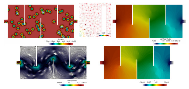
    Flow on a maze-shaped domain. Heterogeneous permeability distribution, zoom to visualize the simplicial barycentric trisected mesh, Cauchy stress magnitude, first post-process of velocity, and post-processed pressure

    .

    In the second 2D example we follow [20] and compute channel flow solutions and take the permeability distribution from the Cartesian SPE10 benchmark dataset for reservoir simulations / model 2 (we choose layer 45, corresponding to a fluvial fan pattern with channeling. See also, e.g., [1,9]). The permeability data has a very large contrast: the minimum and maximum values are and , and it is projected onto a twice quadrisected crisscrossed mesh discretizing the rectangular domain [m]. The remaining parameters are and . On the inlet (the left segment of the boundary) we impose the inflow velocity [m/s], on the outlet (the right vertical segment) we set zero normal stress, and on the horizontal walls we impose no-slip conditions.

    The flow patterns are shown in Figure 2, and the qualitative behaviour coincides with the expected filtration mechanisms observed elsewhere (see, e.g., [22]). The magnitude of velocity in its second post-process , and the stress magnitude are plotted in logarithmic scale.

    Figure 2. 

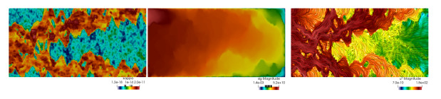
    Channel flow with permeability from the SPE10–layer 45 benchmark data, and using a twice quadrisected crisscrossed mesh. Heterogeneous permeability distribution in log scale, Cauchy stress magnitude in log scale, and line integral convolution of second post-process of velocity in log scale

    .

    3D flow through porous media. To close this section, in this test we use a cylindrical geometry of radius 0.2 [m] and height 0.7 [m], discretized into an unstructured simplicial barycentric quadrisected mesh of 48756 tetrahedra. We set the viscosity to the value of water and again use inlet (the face ), wall (the surface [m]), and outlet (the face [m]) type of boundary conditions mimicking a channel flow with homogeneous right-hand side in the momentum balance . The inlet velocity is . A synthetic permeability field is generated based on a porosity of approximately 0.4. For this we generate a normalized uniform random distribution, apply a Gaussian filter with standard deviation of 2, and then use a quantile of 40%. The resulting field is rescaled between and . Figure 3 presents the permeability and contour iso-surfaces of velocity magnitude, which indicate the formation of wormhole-like structures with higher velocity.

    Figure 3. 

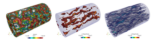
    Channel flow with synthetic permeability. The mesh is of simplicial barycentric quadrisected type. Heterogeneous permeability distribution, contour iso-surfaces of velocity magnitude in log scale, and velocity streamlines

    .

    This research was supported by Spain's Ministry of Economy Project PID2020-116287GB-I00, by the Monash Mathematics Research Fund S05802-3951284, by the Ministry of Science and Higher Education of the Russian Federation within the framework of state support for the creation and development of World-Class Research Centres "Digital biodesign and personalized healthcare" No. 075-15-2022-304, and by the Australian Research Council through the Discovery Project grant DP220103160.


    [1]

    J. E. Aarnes, T. Gimse and K.-A. Lie, An introduction to the numerics of flow in porous media using Matlab, in Geometric Modelling, Numerical Simulation, and Optimization: Applied Mathematics at SINTEF, G. Hasle, K.-A. Lie, and E. Quak, eds., Springer Berlin Heidelberg, Berlin, Heidelberg, 2007, 265-306.

    [2] The FEniCS project version 1.5. Arch. Numer. Softw. (2015) 3: 9-23.
    [3] Analysis of a vorticity-based fully-mixed formulation for the 3D Brinkman-Darcy problem. Comput. Methods Appl. Mech. Engrg. (2016) 307: 68-95.
    [4] An augmented velocity-vorticity-pressure formulation for the Brinkman equations. Int. J. Numer. Methods Fluids (2015) 79: 109-137.
    [5] A priori and a posteriori error analysis of a mixed scheme for the Brinkman problem. Numer. Math. (2016) 133: 781-817.
    [6] Stabilized mixed approximation of axisymmetric Brinkman flows. ESAIM: Math. Model. Numer. Anal. (2015) 49: 855-874.
    [7]

    D. Boffi, F. Brezzi and M. Fortin, Mixed Finite Element Methods and Applications, Springer Series in Computational Mathematics, 44. Springer, Heidelberg, 2013.

    [8] A mixed virtual element method for the Brinkman problem. Math. Models Methods Appl. Sci. (2017) 27: 707-743.
    [9] Tenth SPE comparative solution project: A comparison of upscaling techniques. SPE Reservoir Eval. Engrg. (2001) 4: 308-317.
    [10]

    D. A. Di Pietro and A. Ern, Mathematical Aspects of Discontinuous Galerkin Methods, Springer-Verlag Berlin Heidelberg 2012.

    [11]

    A. Ern and J.-L. Guermond, Finite Elements IIGalerkin Approximation, Elliptic and Mixed PDEs, Texts in Applied Mathematics, Vol. 73, Springer, 2021.

    [12] Finite element quasi-interpolation and best approximation. ESAIM Math. Model. Numer. Anal. (2017) 51: 1367-1385.
    [13]

    R. S. Falk, Finite element methods for linear elasticity, in Mixed Finite Elements, Compatibility Conditions, and Applications, F. Brezzi, D. Boffi, L. Demkowicz, and R. G. Durán, eds., Springer, Berlin 2008,159-194.

    [14] Analysis of a pseudostress-based mixed finite element method for the Brinkman model of porous media flow. Numer. Math. (2014) 126: 635-677.
    [15]

    G. N. Gatica, M. Munar and F. A. Sequeira, A mixed virtual element method for a nonlinear Brinkman model of porous media flow, Calcolo, 55 (2018), Paper No. 21, 36 pp.

    [16] A second elasticity element using the matrix bubble. IMA J. Numer. Anal. (2012) 32: 352-372.
    [17] A family of nonconforming elements for the Brinkman problem. IMA J. Numer. Anal. (2012) 32: 1484-1508.
    [18] Uniformly stable discontinuous Galerkin discretization and robust iterative solution methods for the Brinkman problem. SIAM J. Numer. Anal. (2016) 54: 2750-2774.
    [19] A dual-mixed finite element method for the Brinkman problem. SMAI J. Comput. Math. (2016) 2: 1-17.
    [20] Geometric multigrid for Darcy and Brinkman models of flows in highly heterogeneous porous media: A numerical study. J. Comput. Appl. Math. (2017) 310: 174-185.
    [21] H(div)-conforming finite elements for the Brinkman problem. Math. Models Methods Appl. Sci. (2011) 21: 2227-2248.
    [22] On the importance of the Stokes-Brinkman equations for computing effective permeability in Karst reservoirs. Commun. Comput. Phys. (2011) 10: 1315-1332.
    [23]

    X. Li and W. Xu, Numerical computation of Brinkman flow with stable mixed element method, Math. Prob. Engrg., (2019), ID 7625201, 10 pp.

    [24] Analyses of mixed continuous and discontinuous Galerkin methods for the time harmonic elasticity problem with reduced symmetry. SIAM J. Sci. Comput. (2015) 37: 1909-1933.
    [25]

    S. Meddahi and R. Ruiz-Baier, Symmetric mixed discontinuous Galerkin methods for linear viscoelasticity, preprint, 2022, arXiv: 2203.01662.

    [26]

    Y. Qian, S. Wu and F. Wang, A mixed discontinuous Galerkin method with symmetric stress for Brinkman problem based on the velocity–pseudostress formulation, Comput. Methods Appl. Mech. Engrg., 368 (2020), article 113177, 23 pp.

    [27] Norm estimates for a maximal right inverse of the divergence operator in spaces of piecewise polynomials. RAIRO Modél. Math. Anal. Numér. (1985) 19: 111-143.
    [28] A mixed formulation for the Brinkman problem. SIAM J. Numer. Anal. (2014) 52: 258-281.
    [29]

    F. Wang, S. Wu and J. Xu, A mixed discontinuous Galerkin method for linear elasticity with strongly imposed symmetry, J. Sci. Comput., 83 (2020), Paper No. 2, 17 pp.

    [30] On the constants in -finite element trace inverse inequalities. Computer Methods in Applied Mechanics and Engineering (2003) 192: 2765-2773.
  • This article has been cited by:

    1. Zeinab Gharibi, A weak Galerkin pseudostress-based mixed finite element method on polygonal meshes: application to the Brinkman problem appearing in porous media, 2024, 97, 1017-1398, 1341, 10.1007/s11075-024-01752-9
  • Reader Comments
  • © 2022 the Author(s), licensee AIMS Press. This is an open access article distributed under the terms of the Creative Commons Attribution License (http://creativecommons.org/licenses/by/4.0)
通讯作者: 陈斌, bchen63@163.com
  • 1. 

    沈阳化工大学材料科学与工程学院 沈阳 110142

  1. 本站搜索
  2. 百度学术搜索
  3. 万方数据库搜索
  4. CNKI搜索

Metrics

Article views(1452) PDF downloads(281) Cited by(1)

Other Articles By Authors

/

DownLoad:  Full-Size Img  PowerPoint
Return
Return

Catalog