
Unlike the classical kinetic theory of rarefied gases, where microscopic interactions among gas molecules are described as binary collisions, the modelling of socio-economic phenomena in a multi-agent system naturally requires to consider, in various situations, multiple interactions among the individuals. In this paper, we collect and discuss some examples related to economic and gambling activities. In particular, we focus on a linearisation strategy of the multiple interactions, which greatly simplifies the kinetic description of such systems while maintaining all their essential aggregate features, including the equilibrium distributions.
Citation: Giuseppe Toscani, Andrea Tosin, Mattia Zanella. Kinetic modelling of multiple interactions in socio-economic systems[J]. Networks and Heterogeneous Media, 2020, 15(3): 519-542. doi: 10.3934/nhm.2020029
[1] | Fabio Camilli, Raul De Maio, Andrea Tosin . Transport of measures on networks. Networks and Heterogeneous Media, 2017, 12(2): 191-215. doi: 10.3934/nhm.2017008 |
[2] | Mapundi K. Banda, Michael Herty, Axel Klar . Coupling conditions for gas networks governed by the isothermal Euler equations. Networks and Heterogeneous Media, 2006, 1(2): 295-314. doi: 10.3934/nhm.2006.1.295 |
[3] | Yacine Chitour, Guilherme Mazanti, Mario Sigalotti . Stability of non-autonomous difference equations with applications to transport and wave propagation on networks. Networks and Heterogeneous Media, 2016, 11(4): 563-601. doi: 10.3934/nhm.2016010 |
[4] | Yaojun Liu, Li Jia, Ping Wang, Xiaolin Song . Joint optimization of location and allocation for spare parts depots under ($ r, Q $) inventory policy. Networks and Heterogeneous Media, 2024, 19(3): 1038-1057. doi: 10.3934/nhm.20240046 |
[5] | Fatih Bayazit, Britta Dorn, Marjeta Kramar Fijavž . Asymptotic periodicity of flows in time-depending networks. Networks and Heterogeneous Media, 2013, 8(4): 843-855. doi: 10.3934/nhm.2013.8.843 |
[6] | Eva Barrena, Alicia De-Los-Santos, Gilbert Laporte, Juan A. Mesa . Transferability of collective transportation line networks from a topological and passenger demand perspective. Networks and Heterogeneous Media, 2015, 10(1): 1-16. doi: 10.3934/nhm.2015.10.1 |
[7] | Mary Luz Mouronte, Rosa María Benito . Structural analysis and traffic flow in the transport networks of Madrid. Networks and Heterogeneous Media, 2015, 10(1): 127-148. doi: 10.3934/nhm.2015.10.127 |
[8] | Nastassia Pouradier Duteil . Mean-field limit of collective dynamics with time-varying weights. Networks and Heterogeneous Media, 2022, 17(2): 129-161. doi: 10.3934/nhm.2022001 |
[9] | Qinglan Xia, Shaofeng Xu . On the ramified optimal allocation problem. Networks and Heterogeneous Media, 2013, 8(2): 591-624. doi: 10.3934/nhm.2013.8.591 |
[10] | Klaus-Jochen Engel, Marjeta Kramar Fijavž, Rainer Nagel, Eszter Sikolya . Vertex control of flows in networks. Networks and Heterogeneous Media, 2008, 3(4): 709-722. doi: 10.3934/nhm.2008.3.709 |
Unlike the classical kinetic theory of rarefied gases, where microscopic interactions among gas molecules are described as binary collisions, the modelling of socio-economic phenomena in a multi-agent system naturally requires to consider, in various situations, multiple interactions among the individuals. In this paper, we collect and discuss some examples related to economic and gambling activities. In particular, we focus on a linearisation strategy of the multiple interactions, which greatly simplifies the kinetic description of such systems while maintaining all their essential aggregate features, including the equilibrium distributions.
In recent times there has been an increasing interest in the notion of measure-valued solutions to evolution equations. Compared to standard approaches based on classical and weak solutions, the measure-theoretic setting allows one to better describe some interesting phenomena such as aggregation, congestion and pattern formation in a multiscale perspective. Several of these phenomena occur in applications such as vehicular traffic, data transmission, crowd motion, supply chains, where the state of the system evolves on a network, see e.g. [5,9,13,14,16].
In order to extend the measure-valued approach to these irregular geometric structures, in this paper we study measure-valued solutions to a linear transport process defined on a network. For classical and weak solutions to transport equations on networks we refer the reader for example to [10,14,18].
The measure-valued approach in Euclidean spaces relies on the notion of push-forward of measures along the trajectories of a vector field describing the transport paths [1,6,7,17]. The study of these problems in bounded domains poses additional difficulties, especially concerning the behaviour at the boundaries of the transported measure. For problems on networks similar difficulties arise at the vertexes.
Our analysis is inspired by the results in [11,12], where measure-valued transport equations are studied in a bounded interval. We also refer to [15], where the authors consider instead measure-valued solutions to non-linear transport problems with measure transmission conditions at nodal points, i.e. points where the velocity vanishes.
Consider a network
μ=∫suppμδxdμ(x), | (1) |
where
From (1) it follows that if we are able to define the transport of an atomic measure
∂tμjt+∂x(vj(x)μjt)=0, | (2) |
For
Φjt(x0,0):=x0+∫t0vj(Φjs(x0,0))ds, |
which describes the trajectory issuing from the point
At
This preliminary discussion sketches the main ideas that we intend to follow in order to tackle the global problem on the network. We first consider a local problem, namely a transport equation on each single arc with a measure acting as a source term (boundary condition) at the initial vertex. For this local problem we formulate an appropriate notion of measure-valued solution, for which we give a representation formula taking into account also the mass which flows out of the arc. Then we glue all the solutions on the single arcs by means of appropriate mass distribution rules at the vertexes, thereby constructing the global solution on the network.
In more detail, the paper is organised as follows. In Section 2 we introduce some notations and assumptions for the problem, while in Section 3 we review some basic facts about the measure-theoretic setting in which we will frame our analysis. In Section 4 we study the initial/boundary-value problem for the transport equation on a single bounded interval, which is the prototype of an arc of the network, then in Section 5 we move to the problem on networks. Finally, in Section 6 we construct explicit measure-valued solutions on simple networks, which constitute preliminary examples of the application of our theory to vehicular traffic.
We start by describing the constitutive elements of the problem.
Definition 2.1. (Network). A network
Given a vertex
We denote by
Definition 2.2. (Distribution matrices). For an internal vertex
pikj(t)≥0diO∑j=1pikj(t)=∑j:Vi=πj(0)pikj(t)=1. | (3) |
Here
For a source vertex
pij(t)≥0diO∑j=1pij(t)=∑j:Vi=πj(0)pij(t)=1. | (4) |
Definition 2.3. (Velocity field). On each arc
Definition 2.4. (Initial and boundary data). We prescribe the initial mass distribution over
To define the transport of the initial measure
{∂tμj+∂x(vj(x)μj)=0x∈Ej,t∈(0,T],j∈Jμjt=0=μj0x∈Ej,j∈JμjVi=πj(0)={dIi∑k=1pikj(t)μkVi=πk(1)if i∈Ipij(t)ςiif i∈S, | (5) |
where by
For an internal vertex, the inflow measure is given by the mass flowing in
The detailed study of problem (5) is postponed to Section 5. Before that, we introduce an appropriate measure theoretic setting, see Section 3, and consider preliminarily the problem on a single arc, see Section 4.
We introduce a space of measures with an appropriate norm where we consider the solutions to our measure-valued transport equations. Moreover, since the notion of solution is based on the superposition principle (1), we briefly describe the measure-theoretic setting which guarantees the validity of this formula. We refer for details to [1,2,11,19].
Let
⟨μ,φ⟩:=∫Tφdμ. |
Given a Borel measurable vector field
(Φ#μ)(E):=μ(Φ−1(E)),∀E∈B(T). |
We immediately observe that
Given a metric
||φ||BL:=||ϕ||∞+|ϕ|L, |
where the semi-norm
|φ|L:=supx,y∈Tx≠y|φ(y)−φ(x)|d(x,y). |
Furthermore, we introduce a norm in
‖μ‖∗BL:=supφ∈BL(T)||φ||BL≤1⟨μ,φ⟩. |
It is easy to see that if
The space
Remark 1. If
Remark 2. The distance induced in
||μ||TV:=supφ∈Cb(T)||φ||∞≤1⟨μ,φ⟩, |
where
‖δy−δx‖∗BL≤d(x,y),||δy−δx||TV=2. |
Hence the two measures are closer and closer in the norm
As alredy anticipated in Section 1, for the subsequent development of the theory we will extensively use the following fact linked to the concept of Bochner integral [2,19]: any
μ=∫Tδxdμ(x) |
as a Bochner integral in
We now specialise the previous definitions to the case
d(x,y)+|t−s|,(x,t),(y,s)∈Γ×[0,T], |
We consider the Borel
A measure
For
⟨μ,φ⟩:=∑j∈J∫Ej×[0,T]φdμj. | (6) |
For a function
φ(x,t)=φj(y,t)for x∈Ej, y=π−1j(x), t∈[0,T]. |
A function
||φ||BL(Γ×[0,T]):=supj∈J||φj||BL([0,1]×[0,T]). |
The corresponding dual norm
‖μ‖∗BL:=supφ∈BL(Γ×[0,T])||φ||BL(Γ×[0,T])≤1⟨μ,φ⟩. |
In this section we study the transport equation in a bounded interval. Actually, we start by focusing on the problem of prescribing appropriate initial and boundary conditions to the differential equation in
Consider the conservation law
∂tμ+∂x(v(x)μ)=0,(x,t)∈R+×R+, | (7) |
where
● using the projection with respect to the space variable we can write
μ(dxdt)=μt(dx)⊗dt, | (8) |
where
● similarly, projecting with respect to the time variable we can write
μ(dxdt)=νx(dt)v(x)⊗dx, | (9) |
where
Remark 3. The coefficient
We incidentally notice that if
Relying on the concept of conditional measures, we formulate the following initial/boundary-value problem for (7):
{∂tμ+∂x(v(x)μ)=0(x,t)∈R+×R+μt=0=μ0∈M+(R+0×{0})νx=0=ν0∈M+({0}×R+0) | (10) |
with
● assigning an initial condition at
● assigning a boundary condition at
In order to give a suitable notion of measure-valued solution to (10), we preliminarily introduce integration-by-parts formulas useful to deal with the initial and boundary data. Let
⟨∂tμ,φ⟩:=−⟨μ,∂tφ⟩−∫R+0φ(x,0)dμ0(x),⟨∂x(v(x)μ),φ⟩:=−⟨μ,v(x)∂xφ⟩−∫R+0φ(0,t)dν0(t), |
where
Remark 4. With a slight abuse of notation, in the following we will denote
∫R+0φ(x,0)dμ0(x)=:⟨μ0,φ⟩,∫R+0φ(0,t)dν0(t)=:⟨ν0,φ⟩, |
the difference between duality pairings in
Thanks to these formulas, we are in a position to introduce the following notion of measure-valued solution to (10):
Definition 4.1. Given
⟨μ,∂tφ+v(x)∂xφ⟩=−⟨μ0,φ⟩−⟨ν0,φ⟩,∀φ∈C10(R+0×R+0). | (11) |
Since (10) is a linear problem, its solution can be obtained from the superposition of two measures
However, for the next purposes it is convenient to characterise the solution
μ(dxdt)=(μ1t(dx)+μ2t(dx))⊗dt, |
where
In order to obtain a formula for
{ddtΦt(x,0)=v(Φt(x,0)),t>0Φ0(x,0)=x. | (12) |
By standard results, it is well known that
μ1t=Φt#μ0=∫R+0δΦt(x,0)dμ0(x)∈M+(R+0×{t}), |
where
Likewise, to obtain a formula for
{ddtΦt(0,s)=v(Φt(0,s)),t>sΦs(0,s)=0. | (13) |
By transporting the mass
μ2t=∫[0,t]δΦt(0,s)dν0(s)∈M+(R+0×{t}), |
where the integral is again meant in the sense of Bochner.
Summing up, we consider the following representation formula for
μ(dxdt)=(∫R+0δΦt(ξ,0)(dx)dμ0(ξ)+∫[0,t]δΦt(0,s)(dx)dν0(s))⊗dt | (14) |
and we check that it actually defines a solution to (10) in the sense of Definition 4.1. To this purpose we preliminarily observe that, since
∫R+0f(x)dμ1t(x)=∫R+0f(Φt(x,0))dμ0(x). | (15) |
We can obtain a similar formula for
∫R+0f(x)dμ2t(x)=N∑k=1αkμ2t(Ak)=N∑k=1αk∫[0,t]δΦt(0,s)(Ak)dν0(s)=N∑k=1αk∫[0,t]χAk(Φt(0,s))dν0(s)=∫[0,t]N∑k=1αkχAk(Φt(0,s))dν0(s)=∫[0,t]f(Φt(0,s))dν0(s). |
Approximating a measurable function
∫R+0f(x)dμ2t(x)=∫[0,t]f(Φt(0,s))dν0(s). | (16) |
Interestingly, an integral with respect to the
Plugging (14) into the left-hand side of (11) and using (15), (16) we discover:
⟨μ,∂tφ+v(x)∂xφ⟩=∫R+0∫R+0(∂tφ(Φt(x,0),t)+v(Φt(x,0))∂xφ(Φt(x,0),t))dμ0(x)dt=+∫R+0∫[0,t](∂tφ(Φt(0,s),t)+v(Φt(0,s))∂xφ(Φt(0,s),t))dν0(s)dt=∫R+0∫R+0ddtφ(Φt(x,0),t)dμ0(x)dt+∫R+0∫[0,t]ddtφ(Φt(0,s),t)dν0(s)dt, |
where in the last passage we have invoked (12), (13). By switching the order of integration in view of Fubini-Tonelli's Theorem we further obtain
=∫R+0∫R+0ddtφ(Φt(x,0),t)dtdμ0(x)+∫R+0∫[s,+∞)ddtφ(Φt(0,s),t)dtdν0(s)=∫R+0[φ(Φt(x,0),t)]t=+∞t=0dμ0(x)+∫R+0[φ(Φt(0,s),t)]t=+∞t=sdν0(s)=−∫R+0φ(x,0)dμ0(x)−∫R+0φ(0,s)dν0(s)=−⟨μ0,φ⟩−⟨ν0,φ⟩, |
which confirms that (14) is indeed a measure-valued solution to (10). Uniqueness of such a solution is a consequence of continuous dependence estimates on the initial and boundary data, which can be proved by standard arguments in literature, cf. [1]. In conclusion, for the transport problem in
Theorem 4.2. For
We now pass to consider the transport problem on the bounded domain
{∂tμ+∂x(v(x)μ)=0,(x,t)∈Qμt=0=μ0∈M+([0,1]×{0})νx=0=ν0∈M+({0}×[0,T]) | (17) |
for a given bounded, strictly positive and Lipschitz continuous velocity field
μ⌞Q(E):=μ(E∩Q) |
for every measurable set
In particular, in view of the application of this problem to a network, it is important to characterise the traces of
Let us introduce the following quantities:
τ(x):=inf{t≥0:Φt(x,0)=1},x∈[0,1] | (18) |
σ(s):=inf{t≥s:Φt(0,s)=1},s∈[0,T] | (19) |
corresponding to the time needed to the characteristic line issuing from either
Recalling (14) and using
μT:=∫[0,max{0,τ−1(T)}]δΦT(x,0)dμ0(x)+∫[max{0,σ−1(T)},T]δΦT(0,s)dν0(s) | (20) |
whereas, following the characteristics, we construct the trace on the fibre
ν1:=∫(max{0,τ−1(T)},1]δτ(x)dμ0(x)+∫[0,max{0,σ−1(T)})δσ(s)dν0(s). | (21) |
We incidentally notice that the first term at the right-hand side of (20) is the push-forward of
The relationship between these traces and the transport of
Theorem 4.3. Given
⟨μ⌞Q,∂tφ+v(x)∂xφ⟩=⟨μT−μ0,φ⟩+⟨ν1−ν0,φ⟩,∀φ∈C1(ˉQ), | (22) |
where
Moreover, for
‖μ2T−μ1T‖∗BL+‖ν21−ν11‖∗BL≤C(‖μ20−μ10‖∗BL+‖ν20−ν10‖∗BL). | (23) |
Proof. See Appendix A.
We also give a result about the dependence on time.
Theorem 4.4. Given
‖μt−μt′‖∗BL+‖ν1⌞[0,t]−ν1⌞[0,t′]‖∗BL≤C|t−t′|+ν0([t′,t]) | (24) |
for all
Proof. See Appendix A.
Remark 5. Theorem 4.4 states virtually that the traces
If the boundary datum
In the applications, a Lebesgue-absolutely continuous
In this section we go back to the study of problem (5). In order to make the notation consistent with the one introduced in Section 4, we set
νj0:=μjVi=πj(0),νj1:=μjVi=πj(1) |
and we rewrite (5) as
{∂tμj+∂x(vj(x)μj)=0x∈Ej,t∈(0,T],j∈Jμjt=0=μj0x∈Ej,j∈Jνj0={∑k:Vi=πk(1)pikj(t)νk1if i∈Ipij(t)ςiif i∈S. | (25) |
Let
⟨μj,∂tφ+vj(x)∂xφ⟩=⟨μjT−μj0,φ⟩+⟨νj1−νj0,φ⟩ | (26) |
for every
μjT=∫[0,max{0,τ−1j(T)}]δΦjT(x,0)dμj0(x)+∫[max{0,σ−1j(T)},T]δΦjT(0,s)dνj0(s) | (27) |
νj1=∫(max{0,τ−1j(T)},1]δτj(x)dμj0(x)+∫[0,max{0,σ−1j(T)})δσj(s)dνj0(s), | (28) |
where the flow maps
Summing (26) over
⟨μ,∂tφ+v(x)∂xφ⟩=⟨μT−μ0,φ⟩+∑j∈J⟨νj1−νj0,φ⟩, | (29) |
where
μ0=∑j∈Jμj0,μT=∑j∈JμjT. | (30) |
In particular, the last term at the right-hand side in (29) can be rewritten in more detail by summing on the vertexes of the network:
∑j∈J⟨νj1−νj0,φ⟩=∑i∈I(∑j:Vi=πj(1)⟨νj1,φ⟩−∑j:Vi=πj(0)⟨νj0,φ⟩)=∑i∈I(∑j:Vi=πj(1)⟨νj1,φ⟩−∑j:Vi=πj(0)⟨νj0,φ⟩)=+∑i∈W∑j:Vi=πj(1)⟨νj1,φ⟩−∑i∈S∑j:Vi=πj(0)⟨νj0,φ⟩. |
For an internal vertex
∑j:Vi=πj(1)⟨νj1,φ⟩−∑j:Vi=πj(0)⟨νj0,φ⟩=∑j:Vi=πj(1)⟨νj1,φ⟩=−∑j:Vi=πj(0)⟨∑k:Vi=πk(1)pikj(t)νk1,φ⟩=∑j:Vi=πj(1)⟨νj1,φ⟩=−∑k:Vi=πk(1)⟨∑j:Vi=πj(0)pikj(t)νk1,φ⟩ |
whence, taking (3) into account in the second term at the right-hand side,
=∑j:Vi=πj(1)⟨νj1,φ⟩−∑k:Vi=πk(1)⟨νk1,φ⟩=0. |
This is the conservation of the mass through the internal vertexes of the network.
For a source vertex
∑i∈S∑j:Vi=πj(0)⟨νj0,φ⟩=∑i∈S∑j:Vi=πj(0)⟨pij(t)ςi,φ⟩=∑i∈S⟨(∑j:Vi=πj(0)pij(t))ςi,φ⟩ |
whence, in view of (4),
=∑i∈S⟨ςi,φ⟩=⟨ς,φ⟩ |
where we have defined the measure
Finally, for a well vertex
ωi:=∑j:Vi=πj(1)νj1∈M+({Vi}×[0,T]),ω:=∑i∈Wωi∈M+(∪i∈W{Vi}×[0,T]), | (31) |
which represents the total mass flowing out of the network up to the time
Equation (29) takes then the form
⟨μ,∂tφ+v(x)∂xφ⟩=⟨μT−μ0,φ⟩+⟨ω−ς,φ⟩,∀φ∈C1(Γ×[0,T]), | (32) |
thereby expressing the counterpart of (22) on the network.
Using the formulation just obtained, we are in a position to establish the well-posedness of the transport problem over networks.
Theorem 5.1. Given
Moreover, for
‖μT,2−μT,1‖∗BL+‖ω2−ω1‖∗BL≤C(‖μ0,2−μ0,1‖∗BL+‖ς2−ς1‖∗BL). | (33) |
Proof. We treat separately the cases in which the set of the source vertexes is or is not empty.
(ⅰ) Assume
E0={Ej:Vi=πj(0) is a source}Em={Ej:∃Ek∈Em−1 s.t. Vi=πj(0)=πk(1)},m=1,2,… |
We first apply Theorem 4.3 to the problem defined on each arc in
{∂tμj+∂x(vj(x)μj)=0in Ej×(0,T]μjt=0=μj0∈M+(Ej×{0})νj0=pij(t)ςi∈M+({Vi}×[0,T]). |
Since
{∂tμj+∂x(vj(x)μj)=0in Ej×(0,T]μjt=0=μj0∈M+(Ej×{0})νj0=diI∑k=1pikj(t)νk1∈M+({Vi}×[0,T]). |
Since the arcs
In this way, after a finite number of steps we build arc by arc the measures
(ⅱ) Assume now
t0<minj∈J:Vi=πj(1)τj(0). |
From (28) we see that, up to the time
νj1=∫(τ−1j(t0),1]δτj(x)dμj0(x), |
because
Let us consider the initial/boundary-value problem (25) for
ςi=∑j:Vi=πj(1)νj1=∑j:Vi=πj(1)∫(τ−1j(t0),1]δτj(x)dμj0(x). |
From the case
Finally, the estimate (33) is in both cases an immediate consequence of the corresponding estimate (23) holding on each arc.
In this section we write explicitly the solution to problem (25) for two typical junctions which occur frequently for instance in traffic flow on road networks. It is worth pointing out that, since in our linear equation the velocity depends only on the space variable but not on the measure
Let
where the velocity fields
The solution on each road has the form
Furthermore, using Bochner integrals in the product space
Remark 6. By carefully inspecting the expressions of
Unlike the Dirac delta entering the road
This approach differs from the one proposed in [8], which instead assigns a path to each microscopic vehicle through the network in the spirit of the multipath traffic model introduced in [3,4].
We now consider the same network as in the previous Section 6.1 but we prescribe an inflow measure
where
Recalling that the network is initially empty and using (27), we obtain that for each
where in the last passage we have set
where in the second passage we have set
According to our transmission conditions, this mass is distributed to the outgoing roads
which, owing to (27), implies that the traces
and by
It is interesting to note that, since in general the density
Finally, the outflow masses
and
Observing that
Remark 7. The transport problem being linear, the case of an inflow measure
We consider now the road network
Like in Sections 6.1, 6.2, we assume that the network is initially empty. At two successive time instants
where the velocity fields
Relying again on (27), (28) we write explicitly the solution
whence, using Bochner integrals in the product spaces
Proof of Theorem 4.3 We observe that
We begin by considering the case
(34) |
and we have to show that
(35) |
where
thus for
where in the last passage we have used (12). Switching the order of integration, we continue the calculation as:
From (34) we recognise that the term (ⅰ) is indeed
We consider now the case
(36) |
and we have to show that
(37) |
where
hence for
where in the last passage we have used (13). We now switch the order of integration to discover:
Thanks to (36) we recognise that the term (ⅰ) is
To conclude the proof, we show the continuous dependence estimate (23). We consider two problems of the type (17) with respective initial data
We begin by estimating the term
where here
and consequently, taking the supremum over
Proceeding in a similar way for
hence, taking the supremum over
Summing the two estimates just obtained yields finally (23).
Moreover, for
Proof of Theorem 4.4. We begin with the estimate of
we can write:
Likewise, assuming for simplicity that
Hence
and finally, taking the supremum over
We now consider the estimate on the outflow measures. Taking again
We point out that if
Moreover,
which gives
Therefore
whence, taking the supremum over
Summing the estimates obtained so far for
A.T. is member of GNFM (Gruppo Nazionale per la Fisica Matematica) of INdAM (Istituto Nazionale di Alta Matematica), Italy.
A.T. acknowledges that this work has been written within the activities of a research project funded by "Compagnia di San Paolo" (Turin, Italy).
1. | Giulia Cavagnari, Antonio Marigonda, Benedetto Piccoli, Generalized dynamic programming principle and sparse mean-field control problems, 2020, 481, 0022247X, 123437, 10.1016/j.jmaa.2019.123437 | |
2. | Fabio Camilli, Raul De Maio, Andrea Tosin, Measure-valued solutions to nonlocal transport equations on networks, 2018, 264, 00220396, 7213, 10.1016/j.jde.2018.02.015 | |
3. | Fabio Bagagiolo, Rosario Maggistro, Raffaele Pesenti, Origin-to-destination network flow with path preferences and velocity controls: A mean field game-like approach, 2021, 8, 2164-6066, 359, 10.3934/jdg.2021007 | |
4. | Joseph Andria, Rosario Maggistro, Raffaele Pesenti, Sustainable Management of Tourist Flow Networks: A Mean Field Model, 2023, 196, 0022-3239, 730, 10.1007/s10957-023-02158-8 | |
5. | Fabio Bagagiolo, Silvia Faggian, Rosario Maggistro, Raffaele Pesenti, Optimal Control of the Mean Field Equilibrium for a Pedestrian Tourists’ Flow Model, 2022, 22, 1566-113X, 243, 10.1007/s11067-019-09475-4 | |
6. | SIMONE CACACE, FABIO CAMILLI, RAUL DE MAIO, ANDREA TOSIN, A measure theoretic approach to traffic flow optimisation on networks, 2019, 30, 0956-7925, 1187, 10.1017/S0956792518000621 | |
7. | Diogo A. Gomes, Diego Marcon, Fatimah Al Saleh, 2019, The current method for stationary mean-field games on networks, 978-1-7281-1398-2, 305, 10.1109/CDC40024.2019.9029982 | |
8. | Zlatinka Dimitrova, Flows of Substances in Networks and Network Channels: Selected Results and Applications, 2022, 24, 1099-4300, 1485, 10.3390/e24101485 | |
9. | Fabio Bagagiolo, Raffaele Pesenti, 2017, Chapter 1, 978-3-319-70618-4, 3, 10.1007/978-3-319-70619-1_1 | |
10. | Fabio Camilli, Giulia Cavagnari, Raul De Maio, Benedetto Piccoli, Superposition principle and schemes for measure differential equations, 2021, 14, 1937-5077, 89, 10.3934/krm.2020050 | |
11. | Christian Düll, Piotr Gwiazda, Anna Marciniak-Czochra, Jakub Skrzeczkowski, Measure differential equation with a nonlinear growth/decay term, 2023, 73, 14681218, 103917, 10.1016/j.nonrwa.2023.103917 | |
12. | Antonio Siconolfi, Alfonso Sorrentino, Aubry–Mather theory on graphs, 2023, 36, 0951-7715, 5819, 10.1088/1361-6544/acf6ef |
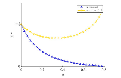
The asymptotic wealth variance
Evolution at times
Comparison between the large time solution (
Comparison between the equilibrium distribution
Evolution at times
Left: comparison of the equilibrium distribution 30 and the large time distribution of the linearised model (22), (24) in the quasi-invariant limit. Right: comparison of the evolution of the energy of the multiple-interaction model (20) with