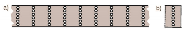
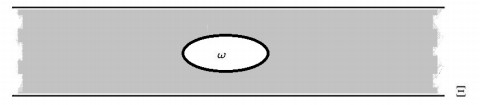
We address a spectral problem for the Dirichlet-Laplace operator in a waveguide $ \Pi^ \varepsilon $. $ \Pi^ \varepsilon$ is obtained from repsilon an unbounded two-dimensional strip $ \Pi $ which is periodically perforated by a family of holes, which are also periodically distributed along a line, the so-called "perforation string". We assume that the two periods are different, namely, $ O(1) $ and $ O( \varepsilon) $ respectively, where $ 0< \varepsilon\ll 1 $. We look at the band-gap structure of the spectrum $ \sigma^ \varepsilon $ as $ \varepsilon\to 0 $. We derive asymptotic formulas for the endpoints of the spectral bands and show that $ \sigma^ \varepsilon $ has a large number of short bands of length $ O( \varepsilon) $ which alternate with wide gaps of width $ O(1) $.
Citation: Sergei A. Nazarov, Rafael Orive-Illera, María-Eugenia Pérez-Martínez. Asymptotic structure of the spectrum in a Dirichlet-strip with double periodic perforations[J]. Networks and Heterogeneous Media, 2019, 14(4): 733-757. doi: 10.3934/nhm.2019029
We address a spectral problem for the Dirichlet-Laplace operator in a waveguide $ \Pi^ \varepsilon $. $ \Pi^ \varepsilon$ is obtained from repsilon an unbounded two-dimensional strip $ \Pi $ which is periodically perforated by a family of holes, which are also periodically distributed along a line, the so-called "perforation string". We assume that the two periods are different, namely, $ O(1) $ and $ O( \varepsilon) $ respectively, where $ 0< \varepsilon\ll 1 $. We look at the band-gap structure of the spectrum $ \sigma^ \varepsilon $ as $ \varepsilon\to 0 $. We derive asymptotic formulas for the endpoints of the spectral bands and show that $ \sigma^ \varepsilon $ has a large number of short bands of length $ O( \varepsilon) $ which alternate with wide gaps of width $ O(1) $.

| [1] |
M. S. Birman and M. Z. Solomjak, Spectral Theory of Selfadjoint Operators in Hilbert Spaces, Mathematics and its Applications (Soviet Series). D. Reidel Publishing Co., Dordrecht, 1987. |
| [2] |
Gap opening and split band edges in waveguides coupled by a periodic system of small windows. Math. Notes (2013) 93: 660-675. 
|
| [3] |
D. I. Borisov and K. V. Pankrashkin, Quantum waveguides with small periodic perturbations: Gaps and edges of Brillouin zones, Journal of Physics A: Mathematical and Theoretical, 46 (2013), 235203, 18 pp. |
| [4] |
C. Conca, J. Planchard and M. Vanninathan, Fluids and Periodic Structures, RAM: Research in Applied Mathematics, 38. John Wiley & Sons, Ltd., Chichester, Masson, Paris, 1995. |
| [5] | A strange term coming from nowhere. Topics in the Mathematical Modelling of Composite Materials, Progr. Nonlinear Differential Equations Appl., Birkhäuser, Boston (1997) 31: 45-93. |
| [6] | Expansion in characteristic functions of an equation with periodic coefficients. Doklady Akad. Nauk SSSR(N.S.) (1950) 73: 1117-1120. |
| [7] |
A boundary value problem for the elliptic equation of second order in a domain with a narrow slit. 1. The two-dimensional case. Math. USSR-Sb. (1976) 28: 459-480.
|
| [8] |
A. M. Il'in, Matching of Asymptotic Expansions of Solutions of Boundary Value Problems, Translations of Mathematical Monographs, 102. American Mathematical Society, Providence, RI, 1992. |
| [9] |
T. Kato, Perturbation Theory for Linear Operators, Die Grundlehren der mathematischen Wissenschaften, Band 132 Springer-Verlag New York, Inc., New York, 1966. |
| [10] | Boundary value problems for elliptic equations in domains with conical or angular points. Trudy Moskov. Mat. Obshch. (1967) 16: 209-292. |
| [11] |
P. Kuchment, Floquet Theory for Partial Differential Equations, Operator Theory: Advances and Applications, 60. Birkhäuser Verlag, Basel, 1993. |
| [12] |
N. S. Landkof, Foundations of Modern Potential Theory, Die Grundlehren der Mathematischen Wissenschaften, Band 180. Springer-Verlag, New York-Heidelberg, 1972. |
| [13] |
D. Leguillon and E. Sánchez-Palencia, Computations of Singular Solutions in Elliptic Problems and Elasticity, John Wiley & Sons, Ltd., Chichester, Masson, Paris, 1987. |
| [14] |
M. Lobo, O. A. Oleinik, E. Perez and T. A. Shaposhnikova, On homogenization of solutions of boundary value problems in domains, perforated along manifolds, Ann. Scuola Norm. Sup. Pisa Cl. Sci. (4), 25 (1998), 611–629. |
| [15] |
M. Lobo and E. Pérez, On the local vibrations for systems with many concentrated masses near the boundary, C.R. Acad. Sci. Paris, Ser. IIb, 324 (1997), 323-329. |
| [16] |
V. A. Marchenko and E. Y. Khruslov, Homogenization of Partial Differential Equations, Progress in Mathematical Physics, 46. Birkhäuser Boston, Inc., Boston, MA, 2006. |
| [17] |
V. Maz'ya, S. Nazarov and B. Plamenevskij, Asymptotic Theory of Elliptic Boundary Value Problems in Singularly Perturbed Domains, Vol. I, Operator Theory: Advances and Applications, 111. Birkhäuser Verlag, Basel, 2000. |
| [18] |
Problème d'écrans perforés pour l'équation de Laplace. RAIRO. Modél. Math. Anal. Numér. (1985) 19: 33-63.
|
| [19] |
Asymptotic conditions at a point, self-adjoint extensions of operators and the method of matched asymptotic expansions. Proceedings of the St. Petersburg Mathematical Society, Vol. V, Amer. Math. Soc. Transl. Ser. 2, Amer. Math. Soc., Providence, RI (1999) 193: 77-125.
|
| [20] |
The polynomial property of self-adjoint elliptic boundary-value problems and the algebraic description of their attributes. Russ. Math. Surveys (1999) 54: 947-1014.
|
| [21] |
Opening of a gap in the continuous spectrum of a periodically perturbed waveguide. Mathematical Notes (2010) 87: 738-756.
|
| [22] |
Asymptotic behavior of spectral gaps in a regularly perturbed periodic waveguide. Vestnik St. Petersburg Univ. Mathematics (2013) 46: 89-97.
|
| [23] |
S. A. Nazarov, R. Orive-Illera and M.-E. Pérez-Martínez, On the polarization matrix for a perforated strip, in Integral Methods in Science and Engineering: Analytic Treatment and Numerical Approximations, Birkhauser, N.Y., (2019), 267–281. |
| [24] |
New asymptotic effects for the spectrum of problems on concentrated masses near the boundary. Comptes Rendues de Mécanique (2009) 337: 585-590.
|
| [25] |
On multi-scale asymptotic structure of eigenfunctions in a boundary value problem with concentrated masses near the boundary. Rev. Mat. Complut. (2018) 31: 1-62.
|
| [26] |
S. A. Nazarov and B. A. Plamenevskii, Elliptic Problems in Domains with Piecewise Smooth Boundaries, De Gruyter Expositions in Mathematics, 13. Walter de Gruyter & Co., Berlin, 1994. |
| [27] |
O. A. Oleinik, A. S. Shamaev and G. A. Yosifia, Mathematical Problems in Elasticity and Homogenization, Studies in Mathematics and its Applications, 26. North-Holland Publishing Co., Amsterdam, 1992. |
| [28] | Higher order asymptotics of solutions of problems on the contact of periodic structures. Mat. Sb. (N.S.) (1979) 110(152): 505-538. |
| [29] |
G. Polya and G. Szegö, Isoperimetric Inequalities in Mathematical Physics, Annals of Mathematics Studies, no. 27, Princeton University Press, Princeton, N. J., 1951. |
| [30] | (1978) Methods of Modern Mathematical Physics. IV. Analysis of Operators. New York-London: Academic Press. |
| [31] |
J. Sanchez-Hubert and E. Sánchez-Palencia, Vibration and Coupling of Continuous Systems. Asymptotic Methods, Springer-Verlag, Berlin, 1989. |
| [32] | Un problème d'ecoulement lent d'un fluide incompressible au travers d'une paroi finement perforée. Homogenization Methods: Theory and Applications in Physics, Collect. Dir. Études Rech. Élec. France, Eyrolles, Paris (1985) 57: 371-400. |
| [33] |
M. M. Skriganov, Geometric and arithmetic methods in the spectral theory of multidimensional periodic operators, Trudy Mat. Inst. Steklov., 171 (1985), 122 pp. |
| [34] |
Band spectrum of the Laplacian on a slab with the Dirichlet boundary condition on a grid. Kyushu J. Math. (2003) 57: 87-116.
|
| [35] |
M. Van Dyke, Perturbation Methods in Fluid Mechanics, Applied Mathematics and Mechanics, Vol. 8 Academic Press, New York-London, 1964. |
Figures(2)
Sergei A. Nazarov, Rafael Orive-Illera, María-Eugenia Pérez-Martínez. Asymptotic structure of the spectrum in a Dirichlet-strip with double periodic perforations[J]. Networks and Heterogeneous Media, 2019, 14(4): 733-757. doi: 10.3934/nhm.2019029

a) The perforated strip
The strip


 DownLoad: