Research article Special Issues

Improved bounds for reaction-diffusion propagation driven by a line of nonlocal diffusion

  • We consider here a model of accelerating fronts, consisting of one equation with nonlocal diffusion on a line, coupled via the boundary condition with a reaction-diffusion equation of the Fisher-KPP type in the upper half-plane. It was proposed in a previous work by H. Berestycki, L. Rossi and the authors, as a mechanism of front acceleration by a line of fast diffusion. In this latter work, it was indeed proved that the propagation in the direction of the line was exponentially fast in time. Inspired by numerical simulations of the first author, we make the estimate more precise by computing a time algebraic correction.

    Citation: Anne-Charline Chalmin, Jean-Michel Roquejoffre. Improved bounds for reaction-diffusion propagation driven by a line of nonlocal diffusion[J]. Mathematics in Engineering, 2021, 3(1): 1-16. doi: 10.3934/mine.2021006

    Related Papers:

    [1] Giuseppe Maria Coclite, Lorenzo di Ruvo . On the initial-boundary value problem for a Kuramoto-Sinelshchikov type equation. Mathematics in Engineering, 2021, 3(4): 1-43. doi: 10.3934/mine.2021036
    [2] Luis A. Caffarelli, Jean-Michel Roquejoffre . The shape of a free boundary driven by a line of fast diffusion. Mathematics in Engineering, 2021, 3(1): 1-25. doi: 10.3934/mine.2021010
    [3] Raúl Ferreira, Arturo de Pablo . A nonlinear diffusion equation with reaction localized in the half-line. Mathematics in Engineering, 2022, 4(3): 1-24. doi: 10.3934/mine.2022024
    [4] Yihong Du, Wenjie Ni . The Fisher-KPP nonlocal diffusion equation with free boundary and radial symmetry in R3. Mathematics in Engineering, 2023, 5(2): 1-26. doi: 10.3934/mine.2023041
    [5] Anoumou Attiogbe, Mouhamed Moustapha Fall, El Hadji Abdoulaye Thiam . Nonlocal diffusion of smooth sets. Mathematics in Engineering, 2022, 4(2): 1-22. doi: 10.3934/mine.2022009
    [6] José Antonio Vélez-Pérez, Panayotis Panayotaros . Wannier functions and discrete NLS equations for nematicons. Mathematics in Engineering, 2019, 1(2): 309-326. doi: 10.3934/mine.2019.2.309
    [7] Gabriele Grillo, Giulia Meglioli, Fabio Punzo . Global existence for reaction-diffusion evolution equations driven by the p-Laplacian on manifolds. Mathematics in Engineering, 2023, 5(3): 1-38. doi: 10.3934/mine.2023070
    [8] Evangelos Latos, Takashi Suzuki . Quasilinear reaction diffusion systems with mass dissipation. Mathematics in Engineering, 2022, 4(5): 1-13. doi: 10.3934/mine.2022042
    [9] Qiang Du, Tadele Mengesha, Xiaochuan Tian . Lp compactness criteria with an application to variational convergence of some nonlocal energy functionals. Mathematics in Engineering, 2023, 5(6): 1-31. doi: 10.3934/mine.2023097
    [10] Serena Della Corte, Antonia Diana, Carlo Mantegazza . Global existence and stability for the modified Mullins–Sekerka and surface diffusion flow. Mathematics in Engineering, 2022, 4(6): 1-104. doi: 10.3934/mine.2022054
  • We consider here a model of accelerating fronts, consisting of one equation with nonlocal diffusion on a line, coupled via the boundary condition with a reaction-diffusion equation of the Fisher-KPP type in the upper half-plane. It was proposed in a previous work by H. Berestycki, L. Rossi and the authors, as a mechanism of front acceleration by a line of fast diffusion. In this latter work, it was indeed proved that the propagation in the direction of the line was exponentially fast in time. Inspired by numerical simulations of the first author, we make the estimate more precise by computing a time algebraic correction.


    This paper is dedicated to S. Salsa, as the expression of our friendship and respect.

    Consider the following system, with unknowns u(t,x) and v(t,x,y), where (t,x,y)R+×R×R+

    {tvΔv=f(v),t>0,xR, y>0,tu+(xx)αu=μu+νvt>0,xR, y=0, t>0yv=μuνv,t>0,xR, y=0. (1.1)

    The real number μ is a positive given parameter, and the nonlinear term f is chosen as

    f(v)=avg(v),

    with a>0 and g of class C2, with g0, convex, g(0)=g(0)=0, g(+)>a. The equation for v in the upper half-plane is therefore a variant of the Fisher-KPP equation, in reference to the pioneering works of Fisher [11] and of Kolmogorov, Petrovskii and Piskunov [14]. The operator (xx)α is the fractional Laplacian of order α(0,1):

    (xx)αu(x)=cα P.V.(Ru(y)u(x)|xy|1+2αdy),

    the constant cα>0 being chosen so that the symbol of (xx)α is |ξ|1+2α. By P. V. we mean

    limε0(|xy|εu(y)u(x)|xy|1+2αdy),

    an expression that is well defined as soon as u is bounded on R, and smooth enough.

    The initial datum is chosen as

    (u(0,x),v(0,x,y))=(δ01(x0,x0)(x),0) (1.2)

    where x0 and δ0 are given positive constants. Their value is not relevant for the discussion, one may think them as small. Under the listed assumptions, system (1.1) has a unique global smooth solution, that is also globally bounded as well as its derivatives, see [2]. The question under study is the behaviour of (u(t,x),v(t,x,y)) for large t.

    System (1.1) is relevant in the study of the influence of a line having a fast diffusion of its own, that exchanges with an adjacent domain of the plane (here, the upper half plane), in which reactive and diffusive phenomena occur. The application is the modelling of how biological invasions can be enhanced by transportation networks, see [4] for an overview. In this context, u(t,x) represents the density of individuals on the line, and v(t,x,y) represents the density of individuals in the upper half-plane. Exchanges occur through the Robin condition yv(t,x,0)=μu(t,x)νv(t,x,0).

    System (1.1) was first introduced by H. Berestycki, L. Rossi and the second author in [7]. There, the diffusion on the line (that we called "the road", while the upper half plane was called "the field") took the form Dxx, with D>0, possibly large. The effect of the line may be accounted for as follows: when not present, the model amounts to the single Fisher-KPP equation with unknown v(t,X), XR2:

    {vtΔv=f(v),t>0, XR2v(0,X)=δ01(x0,x0)2(X),XR2. (1.3)

    Note that here, we need to shift the mass from the line to the plane in order to avoid the trivial solution v0. We have (Aronson, Weinberger [1])

    for all ε>0,limt+inf|X|(cε)tv(t,X)=v0for all ε>0,limt+sup|X|(c+ε)tv(t,X)=0, (1.4)

    where c=2a, and v0 is the unique positive zero of f, whose existence is granted by the assumptions. In other words, the stable state v0 invades the whole space at speed c. Reverting to (1.1), and concentrating on what happens on the line (or its vicinity), first when the diffusion is Dxx, then when it is (xx)α. In the first case, the main result of [7] is the existence of c(D)>0, with lim infc(D)D>0, such that invasion occurs at speed c(D) on the line and in the upper half plane, at finite distance from the line. This shows the importance of the line on the overall propagation. The limiting states for u and v are uνv0μ, vv0, a property that is not entirely trivial, and also proved in [7].

    The effect of the nonlocal diffusion (xx)α was studied for the first time in [2] by H. Berestycki, L. Rossi and the two authors of the present paper. The main result of [2] is the following.

    Theorem 1.1. Define λ=a1+2α. Then we have

    for all ε>0,limt+inf|x|e(λε)t(u(t,x),v(t,x,y))=(νv0μ,v0)for all ε>0,limt+sup|x|e(λ+ε)t(u(t,x),v(t,x,y))=0. (1.5)

    In (1.5), the limits of v should be understood pointwise in y.

    Let us note that this result may be parallelled by the following one: let us bluntly replace the exchange term μuνv in the equation for u by the reaction term f(u) (so that we shift the whole weight of the reaction from the upper half plane to the line), so as to obtain

    {ut+(xx)αu=f(u)(t>0, xR)u(0,x)=δ01(x0,x0)(x). (1.6)

    Then, Cabré and the second author [8] proved that invasion at the same rate as in Theorem 1.1 occurs. Thus, u(t,x) actually behaves just as in equation (1.6) at the leading order.

    While Theorem 1.1 captures the essence of the main features of the invasion phenomenon, it is interesting to ask whether the asymptotics can be made a little more precise. Indeed there is, in Theorem 1.1, a lot of room between the upper and lower bound. For instance the level sets of u may advance like tpeλt, where p could be any real number. This question can also be asked for the simpler model (1.6), all the more as one may give the following heuristics: the dynamics of (1.6) being driven by the small values of u (given the concavity of u they are, loosely speaking, the most unstable ones in the range of f), so that the dynamics of the level sets is really given by the linear equation

    ut+(xx)αu=au.

    Call Gα(t,x) the fractional heat kernel, we have Gα(t,x)t|x|1+2α for large t and x, see [15] for instance. Then we have

    u(t,x)teat|x|1+2α,

    still for large t and x. So, a level set of u will move like t11+2αeat1+2α. This heuristics does not give the correct sharper behaviour, as was proved by Cabré and the two authors of the paper [9]: a level set {x(t)} of u will in fact be such that |x(t)|eat1+2α is bounded, that is, there is no polynomial correction in the expansion of x(t).

    Consider now the linearised version of (1.1):

    {tvΔv=av,t>0,xR, y>0,tu+(xx)αu=μu+νvt>0,xR, y=0, t>0yv=μuνv,t>0,xR, y=0. (1.7)

    Let us call this time Gα(t,x) the solution u(t,x) with the initial datum δx=0, that is, the u-component of the fundamental solution. Then the first author proved [10] (a more precise estimate will be stated later).

    Gα(t,x)eatt32|x|1+2α,t+, |x|+.

    And so, a level set {x(t)} of the solution u(t,x) of (1.7) will move like t32(1+2α)eat1+2α. The question that we want to address in this paper is whether a discrepancy of the same kind holds between the linear and nonlinear equation.

    Surprisingly, and in contrast to what happens with (1.6), the linear equation (1.7) mimicks the behaviour of the nonlinear one (1.1) in a better fashion than for the fractional Fisher-KPP equation. The result that we are going to prove is the following.

    Theorem 1.2. Consider any λ(0,νv0μ). Let xλ(t) be the largest x such that u(t,x)=λ or u(t,x)=λ. Then, for all δ>0, there is Tλ,δ>0 such that, for all tTλ,δ we have

    ea1+2αtt32(1+2α)+δx(t)ea1+2αtt32(1+2α)δ (1.8)

    In fact, the upper bound is more precise, as we may choose δ=0 there. To improve the lower bound seems to us more challenging, and will be addressed in a future work.

    The paper is organised as follows. In Section 2, we explain the strategy of the proof of Theorem 1.2 and discuss some perspectives that our work has opened. In Section 3 we address the underlying mechanism of Theorem 1.2, namely, the transients of the one-dimensional Fisher-KPP equation with Dirichlet boundary conditions, this is a result of independent interest for the Fisher-KPP equation. We then devote a short section to quantify how the exchanges between the road and the field are organised. The proof of Theorem 1.2 is then displayed in Section 5. In the whole paper, the computations will be greatly simplified when we take a function g0, smooth, convex, supported in (θ,1] for some θ(0,1), with g(1)=1. Therefore, the computations will sometimes be carried out with this type of nonlinearity in order to highlight the main ideas, before being extended to the general Fisher-KPP nonlinearity. Also, from now on we will assume, without loss of generality, that a=1.

    The starting point of this paper was the following numerical simulations, carried out in the PhD thesis of the first author [10]. We take a=1. The Figure 1, taken from [10], represents the graph, at various times, of the function

    xu(t,tmet1+2αx),
    Figure 1.  The different renormalisations.

    that is, the solution u(t,x) with different renormalisations. From left to right, the value of m is m=0, m=32(1+2α) and m=31+2α. The gradation of colours from blue to red represents the advance in time, blue standing for the earlier stages of the development.

    One sees that, on the left, the graph of the renormalised solution tends to spread, whereas, on the right, it becomes a peak at x=0. In the middle, it converges to a nontrivial graph. This indicates a stabilisation mechanism for the middle value of m, and this came to us as a surprise. However, this suggests the following idea: the t3/2 term being typical of the one-dimensional Dirichlet heat equation, we thought that it was interesting to understand this feature in a little more depth.

    Assuming – which will turn out to be a good approximation – that xxv is small, this suggests in fact that, for a fixed x, the function v(t,x,y) behaves like a solution of the one dimensional Fisher-KPP equation

    wtwyy=f(v),t>0, y>0w(t,0)=0,

    This is even more evident when one takes f(v)=avg(v), g vanishing on a small interval to the right of 0. The initial value (or, at least, the value of v at any small positive time) is small, dictated by the size of u(1,x). The Dirichlet boundary condition is the most convenient one that allows to put below the solution v(t,x,y) of (1.1) a barrier devised on the model of w(t,y), with an initial datum suitably dictated by the behaviour of u(t,x) (the solution of (1.1) on the line) at infinity. Of course, with this particular condition, the role of the line seems to be forgotten, such is not exactly the case, as long as we prove – as will be done in the course of this work – some easy lemmas that describe how the communication between the road and the field is organised.

    Let us briefly discuss the optimality of our estimates. Of course, the corrections of the exponents in (1.8) by a small δ>0 shows that there is still a room for improvement. In particular, one could ask whether replacing the Dirichlet boundary condition by the exchange condition yv+νv=μu in the 1D Fisher-KPP equation would lead to the optimal bounds. In fact, the best strategy would probably be to investigate the full one-dimensional problem with unknowns (u(t),v(t,y))

    {vtvyy=f(v),t>0, y>0vy(t,0)=μu(t)νv(t,0)t>0˙u(t)=νv(t,0)μu(t).

    We choose no to do it here, as it would involve, in our opinion, heavier computations with possibly no real further understanding of the mechanisms at work. So, we leave this task for a future contribution.

    In this section we consider a function g0, smooth, convex, supported in (θ,1], with g(1)=1 (this last assumption is in fact unnecessary). Pick a small ε>0 with ε<θ. The goal of this section is to understand how much time it will take to the solution of the model Fisher-KPP equation

    {vtvyy=vg(v)(t>0, y0)v(0,y)=ε1[1/2,1](y)v(t,0)=0 (3.1)

    to reach the value θ at finite distance from y=0. First, let us note that the value θ will eventually be reached at a distance that remains bounded and bounded away from y=0, uniformly with respect to t and ε. Indeed, a classical sub-solution argument (see for instance Berestycki-Hamel-Roques [6]) implies that v will converge to the unique nontrivial solution v of

    v=vg(v)(y>0)v(0)=0, (3.2)

    which satisfies v(0)>0, hence uniformly bounded from below on every set of the form [y0,+), y0>0. On the other hand, as ε0, the time that it will take to v to come close to v will grow infinitely, and our aim is to devise an upper bound that will be precise up to algebraic powers of ε.

    Theorem 3.1. Let vε be the solution to (3.1), and ε<λ<v(1). Define Tε as the first time t such that

    vε(t,1)=λ. (3.3)

    Then, for all δ>0, there is Qδ>0, possibly blowing up as δ0, such that

    eTεT32+δεQδε. (3.4)

    It is worth saying a word on the scenario leading to (3.4), and the special structure of the nonlinearity f(v)=vg(v) will make it especially obvious: the region where the solution will first reach a nontrivial value is not close to 0, but at a large distance from 0. At this stage, one could think of invoking classical results on Fisher-KPP propagation for studying how much more time vε will take to be nontrivial near y=0. This is not the correct intuition, because it would lead to a Tε that would be largely over-estimated. The mechanism is in fact closer to that of nonlocal Fisher-KPP propagation [8,9]. It is also not so far from what happens with the classical Fisher-KPP with slowly decreasing initial data, [12,13].

    Proof of Theorem 3.1. For small, or, even, finite t, (for instance t[1,2]) we have vε(t,y)<θ as soon as ε>0 is small enough. Let us make this assumption; as soon as vεθ everywhere we have g(vε)0 and, thus:

    vε(t,y)=εet112e(yy)24te(y+y)24t4πtdy. (3.5)

    For t1 and y[12,1] we have for all y>1

    e(yy)24te(y+y)24tCyytey25t,

    C>0 universal. So we have, for a possibly different C>0:

    vε(t,y)Cεett.ytey25t. (3.6)

    For all fixed t2, the maximum in y of the right handside of (3.6) is taken at

    y=z0t,

    where z0 is the point of maximum of m(z):=zez2/5. Call m0 the (easily computable) maximum of m, a sufficient condition to have vε(t,y)θ everywhere is to have, from (3.6):

    Cm0εettθ.

    Define T1ε2 as

    eT1εT1ε=θm0Cε. (3.7)

    So, we have easily proved that vε reaches a nontrivial value in a time of (roughly) the order of ln(ε1), but this value is reached at y(lnε1)1/2. To study what happens at finite distance to y=0, consider L>0 large. There is cL>0, with, in the worst case scenario

    limL+cL=0,

    such that, in the limit ε0, we have, from (3.5):

    vε(T1ε,y)cLT1ε, for 1yL. (3.8)

    Let eL(y) be the first Dirichlet eigenfunction of xx on (1,L), we normalise so that its maximum is 1. Thus we have

    eL(y)=sin(πL1(y1)),

    with first eigenvalue

    λ1(L)=π2(L1)2.

    Let v_ε,L(t,y) solve

    (txx1)v_ε,L=0(t>T1ε, y(1,L))v_ε,L(t,1)=v_ε,L(t,L)=0(tT1ε)v_ε,L(T1ε,y)=cLT1εeL(y). (3.9)

    On the one hand, we have

    v_ε,L(t,y)=cLe(1λ1(L))(tT1ε)Tε1eL(y). (3.10)

    On the other hand we have v_ε,L(t,y)vε(t,y) for tT1ε, as long as v_ε,L(t,y) is globally less than θ. This last condition is fulfilled as long as

    tT1ε12(1λ1(L))ln(θ2Tε1cL), (3.11)

    and the maximum is exactly θ at equality. Note that it is attained far away from the origin, that is, at yL=L12+1. However, the situation is not as bad as before, because we now have

    eL(y)πL1(y1), for y1<<L.

    This is certainly a small quantity, but it is independent of ε. Let us set

    T2ε=T1ε+12(1λ1(L))ln(θ2T1ε). (3.12)

    We have now, from (3.11):

    vε(T2ε,y)θπL1(y1),for y<<L.

    From now on, once again by a classical sub-solution argument, there is ˜TL>0 (independent of ε), blowing up as L+, such that

    vε(T1ε+T2ε+˜TL,2)=λ.

    This is not exactly (3.3), but we are now quite close to it: from the Harnack inequality we have

    vε(T1ε+T2ε+˜TL+1,1)qλ,

    for some universal q>0, and the same sub-solution argument yields the (3.3), at a time of the form T1ε+T2ε+˜TL+˜TL, the new constant ˜TL being ε-indeendent. Set Tε=T1ε+T2ε+˜TL+˜TL; it now suffices to notice that (3.11) implies that

    Tε=T1ε+12(1+O(1L2))ln(θ2Tε1cL)+˜TL+˜TL,

    which, combined to (3.7), implies

    1ε=cLeTε˜TLθ1+O(1/L2)T3/2+O(1/L2)ε(1+T1εlnTεT1ε(˜TL+˜TL)).

    Let us denote by μL a common bound for the two O(1L2) appearing in the above expression. We now pick a small δ and choose L>0, denoted by Lδ, such that

    μLδ=δ,Qδ=e˜TLδθ1+δμLδ,

    which is exactly (3.4).

    Remark 3.2 Using f(v)v, and the solution ¯v(t,x) of (3.1) with f(v)=vg(v) replaced by v, we obtain the (sharper) converse inequality

    eTεT3/2εCε,

    thus an asymptotic expansion of Tε:

    Tε=ln1ε+32lnln(1ε)+oε0(lnln(1ε)).

    The goal of this section is to prove that, if the solution on the road is of a certain order at some time and on a certain interval, then the solution in the field will be of the same order, possibly in a square with a smaller size and a little later in time. We also want to prove that the converse holds: if the solution is of some order at some time and some point in the field, this is transmitted to the road. Such results can be seen as weak versions of the Harnack inequality (a bound at a certain time and point would entail the same bound in a whole neighbourhood, possibly at later times) but this will be sufficient for our purpose. See [5] for estimates that are more in the spirit of the Harnack inequality.

    Lemma 4.1. Consider t01, x0R, L1 and ε>0 (not necessarily small) such that

    u(t0,x)ε on [x0L,x0+L].

    There is cL>0 (universal otherwise) such that

    v(t,x,y)cLε on [t0+1,t0+2]×[x0L,x0+L] {×[0,1].}

    Proof. Without loss of generality, we may translate time and space so as to have t0=1, x0=0. Notice then that, because v(t,x,0)0 we have

    ut+(xx)αu+μu0,t1, xR.

    Recall that the fundamental solution of the fractional heat equation of order α, that we call Gα(t,x), is uniformly bounded away from 0 on [1,2]×[L1,L+1]. Thus

    u(t,x)eμ(t1)|y|1Gα(t,xx)u(1,x)dx, for t>1 and |x|L.

    This implies

    u(t,x)cLε, for t[1/2,2] and |x|L.

    Then, recall that f(v)v is bounded from below - say, by Λ>0, with Λ>0, and that

    ˜v(t,x,y)=eΛtv(t,x,y)

    is a super-solution to the heat equation, while the boundary condition reads

    y˜v+ν˜vcLε1[2L,2L](x),

    for a possibly different cL. Thus we have ˜vv_, where

    (tΔ)v_=0(t(1,2],xR,y>0)yv_+νv_=cLε1[2L,2L](x),y=0v_(1,x,y)=0.

    By parabolic regularity we have, for some universal C>0:

    |v_(t,x,y)|Cε,t[1/2,2],|x|3L/2,0y1.

    Thus, there is y0(0,1), independent of x0 - and thus of ε such that

    v_(t,x,y0)cL2ε,1/2t1,x03L/2xx0+3L/2.

    And the classical parabolic Harnack inequality implies the lemma. Note that, due to [3], Section 3, one may push it to the boundary thanks to the Robin condition, at the expense of considering ˜v_(t,x,y):=eνyv_(t,x,y).

    Lemma 4.2. Consider t01, x0R, and ε>0 such that

    v(t0,x0,1)ε.

    For all L>0, there is cL>0 (universal otherwise) such that

    u(t,x),v(t,x,y)cLε on [t0+1,t0+2]×[x02L,x0+2L]×[0,1].

    Proof. Once again there is no loss in generality by assuming t0=1, x0=0. The classical Harnack inequality applied to v entails a lower bound of the order ε at least for v(t,x,1) for t[1,2] and 2Lx2L. Fix now L>0, for all δ(0,1) there is cδ>0 (we omit the dependence in L) such that

    v(t,x,y)cδε,(t,x,y)[1,2]×[L,L]×[δ,1].

    Assume the existence of x1[L,L] and t1[1,2] such that v(t1,x1,0) is much smaller than its order of magnitude in the field. This is equivalent to assuming the existence of a sequence of solutions (un,vn) of (1.1), such that the following situation holds:

    ● for t[1,2], x[x1L/2,x1+L/2] and y=1, then vn(t,x,y)cε (dependence on L omitted),

    ● there is t1[1,2] such that vn(t1,x1,0)1/n.

    Remember that vn is uniformly bounded from above. So, by parabolic regularity, (a subsequence of) the sequence (un,vn)n converges, on [1,2]×[x1L/2,x1+L/2]×[0,1] to a limiting function (u,v) which is not identically equal to 0 due to the first assumption on vn. The Hopf Lemma implies yv(t,x,0)>0, thus the exchange condition yields

    μu(t1,x1)νv(t1,x1,0)<0.

    This contradicts the fact that v(t1,x1,0)=0. Now, we have u(t,x)u_(t,x), with

    {u_t+(xx)αu_+μu_=νcε1[L,L](x),t>0, xRu_(0,x)=0.

    Thus, for t[1,2] we have

    u(t,x)cεeμt10LLGα(ts,xx)dxdscε

    for a constant c that only depends on L.

    The starting point of the analysis is the (computationally non trivial) result, whose main line of the proof are given in [2], and proved in full length in [10]. From now on we will assume, for simplicity, that ν=1.

    Theorem 5.1 ([10], Chapter 4). Let (¯u(t,x),¯v(t,x,y)) solve

    {t¯vΔ¯v=¯v,t>0,xR,y>0t¯u+(xx)α¯u=μ¯u+¯vk¯u,t>0,xRy¯v=μ¯uv,t>0,R,y=0, (5.1)

    with (¯u(0,x),¯v(0,x,y))=(u0(x),0) and u00 nonnegative and compactly supported. There exists a function R(t,x) and constants δ>0, C>0 such that

    1). we have, for large x:

    |¯u(t,x)8αμsin(απ)Γ(2α)Γ(3/2)πett3/2|x|1+2α|R(t,x), (5.2)

    2). and the function R(t,x) is estimated as

    0R(t,x)C(eδt+et|x|min(1+4α,3)+et|x|1+2αt52).

    Note that this result readily entails the upper bound in Theorem 1.2, so that it suffices to prove the lower bound. We first prove it when g is compactly supported in (0,1], then indicate the necessary changes for a general g.

    Assume g to be supported in (θ,1). Let us pick λ(ε,1/μ) and x0>0 (the same argument would apply for x0<0) very large, we set

    u(1,x0):=ε.

    From Theorem 5.1, applied at time t=1, the function u(1,x) is of the order ε (and also of the order 1/x1+2α0) on any interval around x0 whose length will not exceed, say, x0. Thus, from Lemma 4.1, applied on every sub-interval of [x0x0,x0+x0] of length 1 we have

    v(1,x,y)cε for (x,y)[x0x0,x0+x0]×[0,1]. (5.3)

    Note that the constant c does not depend on x0, Lemma 4.1 being purely local.

    We ask how much time it will take for u to reach the value λ at x0. From (5.2) we have, as soon as ε<θ is small enough - that is, if x0 is large enough - and for all L>0:

    u(1/2,x)cLεfor all x[x02L,x0+2L].

    Then, translate the point (x0,0) to the origin, and let this time v_(t,x,y) solve the two-dimensional Fisher-KPP equation with Dirichlet conditions on the road:

    {(tΔ1)v+g(v)=0,t1,xR,y>0v_(t,x,0)=0,t1, xRv_(1,x,y)=cε1[x0,x0](x)1[0,1](y). (5.4)

    As long as v_θ everywhere, it solves the linear equation, that is, with g(v)=0. In such a case it consists of the product of two solutions of the heat equation times the exponential:

    v_(t,x,y)=v_1D(t,y)πt([x0,x0]e(xx)2/4tdx), (5.5)

    where v_1D(t,y) is the solution of the Dirichlet heat equation in y, and is exactly given by (3.5). The function v1D reaches θ in a time T1ε given by equation (3.7), in other words

    T1ε=O(ln(1ε)).

    This time is too short for the solution of the heat equation in x to decay significantly on, say, the interval [L,L] with L large but finite (any size L which is an o(x0) will do). We have indeed, for |x|L and tT1ε:

    1tx0x0e(xx)24tdxC(x0L)22t(x0+L)22teξ2dξC,

    simply because x0ε1/(1+2α) and T1ε is of the order ln(1ε). Thus, the function yv_(T1ε,0,y) reaches a maximum of the order θ, at a point of the order T1ε, while it is of the order 1T1ε for y1. Then, we run (5.4) again, from T1ε, with

    v_(T1ε,x,y)=1[L,L](x)1[1,L]eL(x,y)T1ε,

    the function eL(x,y) being the first eigenfunction of the Dirichlet Laplacian in the rectangle (L,L)×(1,L), and L a large number (in fact we could take L=L). We have

    eL(x,y)=sin(π2Lx)sin(πL1(y1)),

    the first eigenvalue being still an O(1L2). And so, for a time Tε given by (3.12), there is q>0 independent of ε such that v_(Tε,0,1)q.

    To conclude the proof, it remains to prove the existence of q>0 universal such that u(Tε,0)q. This is, however, easy: because x0 is arbitrary, we have

    v(Tε,x,1)qfor x0Lxx0+L,

    and Lemma 4.2 implies the desired bound for u.

    We write again

    f(v)=vg(v),g(0)=g(0)=0, g(1)=1, g>0 on [0,1].

    Thus we have, for all v[0,1]: g(v)=O(v2), and this is what we will really use. In view of what we have already done when g vanishes in a vicinity of 0, what we really have to do is study the function v(t,x,y) solving

    vtΔvv=g(v)(t>0,x>0,y>0)v(t,x,0)=0v(0,x,y)=cε1[x0,x0](x)1[0,1](y):=εv0(x,y), (5.6)

    with ε=11+x1+2α0. In view of the proof of Theorem 3.1, and Section 4, the main property that we have to prove is the following.

    Lemma 5.2. Let T1ε be given by (3.7). There is q>0 universal such that

    v(T1ε,0,1)qTε1. (5.7)

    It then suffices, as in the preceding section, to put v above the solution v_δ,L,L of

    {(tΔ(1δ))vδ,L,L=0(t>T1ε,L<x<L,1<y<L)vδ,L,L(t,x,y)=0(t>0,(x,y)([L,L]×[1,L]))vδ,L,L(0,x,y)=qT1εeL,L(x,y),

    with δ small, and eL,L(y) the first eigenfunction of the Dirichlet Laplacian in (L,L)×(1,L). At time

    T2ε=T1ε+(12+O(δ)+O(1L2)+O(1L2))lnT1ε,

    we have v_δ,L,L(t,x,y)Cδ on (L,L)×(1,L), and one finishes the proof of Theorem 1.2 by Lemmas 4.1 and 4.2.

    Let us therefore present the

    Proof of Lemma 5.2. Call X=(x,y)R×R+ a generic point of the upper half-plane R×R. Let G(t,X,X) be the fundamental solution of the Dirichlet heat equation in the upper half-plane, we have

    G(t,X,X)=G0(t,y,y)G1(t,x),

    the function G0 being the Dirichlet fundamental solution (see (3.5)) whereas G1 is the standard Gaussian G1(t,x)=ex2/4t4πt. The Duhamel formula yields

    v(t,X)=εetR2+G(t,X,X)v0(X)dXt0R2+etsG(ts,X,X)g(v(s,X))dsdX. (5.8)

    We have

    v(s,X)esεR2+G(s,X,X)v0(X)dX.

    We call etsD(ts,s,X,X) the integrand of the second integral in the right handside of (5.8). Because g(v)=O(v2) we get, taking (5.5) and (3.6) into account:

    D(ts,s,X,X)Cε2G(ts,X,X)y2e2y2/5s(1+s3)e2s,

    C>0 universal. Note that we have only estimated the integral for s1, the integral for s1 being negligible. Integrating in x and specialising at x=0 we get

    t0R2+etsG(ts,X,X)g(v(s,X))dsdXCε2t0R+et+sE(ts,s,y)dsdy,

    where

    E(ts,s,y)|1+y|3e(1+y)2/4(ts)ey2/3s(1+|ts|)(ts)1/2s(1+s2). (5.9)

    We are going to prove the inequality

    Tε10R×R+eTε1sD(Tε1s,s,(0,1),X)dsdXC(ε+1Tε1)1Tε1, (5.10)

    C>0 universal. There is nothing special about the point X=(0,1) the inequality would be valid for all neighbouring points, at the expense of increasing C. Recall the inequality (see Sections 2 and 3) for v:

    v1D(Tε1,1)qTε1.

    This, combined to (5.10), will imply the lemma. As we will set, eventually, t=Tε1, we will always assume t large, and

    t=O(ln1ε).

    we cut the time interval (0,t) into two.

    1). s(0,κt), κ>0 small. We will use the factor ey2/3s to make the integral convergent, and make the change of variables yz=y/s.Thus we have

    E(ts,s,y)(1+|z|3)ez2/3(1+(ts))tss,

    using et+se(1+κ)t, the fact that tTε1 and the definition of Tε1, we end up with

    κt0R×R+etsD(ts,s,(0,1),X)dsdXε2te(1+κ)tt3/2.

    And so letting tTε1 we obtain

    (1+κ)Tε10R×R+eTε1D(Tε1,s,(0,1),X)dsdXε12κT1ε. (5.11)

    2). The range sκt. This time we rely on the part e(1+y)24(ts) to make the spatial integral convergent, and we will have to be a little careful about the et+s factor. As for the powers y2, we dominate them by 1+|1+y|2. We make the change of variables yzts and we have

    etsD(t,s,(0,1),X)ε2G1(ts,x)et+sez24ts(1+|z|3)s3ε2G1(ts,x)et+sez24t3ts.

    We integrate on (κt,t)×R×R+. This yields

    tκtR×R+etsD(t,s,(0,1),X)dsdXCε2ett3tκttsesdsCε2e2tt3(1κ)t0σeσdσCTε1.

    Making sure that κ(0,1/4) and putting everything together yields (5.10), hence the lemma.

    The research leading to these results has received funding from the ERC under the European Union's Seventh Frame work Programme (FP/2007-2013) / ERC Grant Agreement 321186 - ReaDi.

    All authors declare no conflicts of interest in this paper.


    [1] Aronson DG, Weinberger HF (1978) Multidimensional nonlinear diffusions arising in population genetics. Adv Math 30: 33-76.
    [2] Berestycki H, Coulon AC, Roquejoffre JM, et al. (2015) The effect of a line with non-local diffusion on Fisher-KPP propagation. Math Mod Meth Appl S 25: 2519-2562.
    [3] Berestycki H, Caffarelli LA, Nirenberg L (1990) Uniform estimates for the regularization of free boundary problems, In: Analysis and Partial Differential Equations, New York: Dekker, 567-619.
    [4] Berestycki H, Coulon AC, Roquejoffre JM, et al. (2014) Speed-up of reaction fronts by a line of fast diffusion, In: Séminaire Laurent Schwartz, Equations aux Dérivés Partielles et Applications, 2013-2014, Ecole Polytechnique, Palaiseau.
    [5] Berestycki H, Ducasse R, Rossi L (2020) Generalized principal eigenvalues for heterogeneous road-field systems. Commun Contemp Math 22: 1950013.
    [6] Berestycki H, Hamel F, Roques L (2005) Analysis of the periodically fragmented environment model: Ⅰ - Species persistence. J Math Biol 51: 75-113.
    [7] Berestycki H, Roquejoffre JM, Rossi L (2013) The influence of a line with fast diffusion on FisherKPP propagation. J Math Biol 66: 743-766.
    [8] Cabre X, Roquejoffre JM (2013) The influence of fractional diffusion on front propagation in Fisher-KPP equations. Commun Math Phys 320: 679-722.
    [9] Cabre X, Coulon AC, Roquejoffre JM (2012) Propagation in Fisher-KPP type equations with fractional laplacian in periodic media. C R Acad Sci Paris 350: 885-890.
    [10] Coulon Chalmin AC, Fast propagation in reaction-diffusion equations with fractional diffusion, PhD thesis, 2014. Available from: thesesups.ups-tlse.fr/2427/.
    [11] Fisher RA (1937) The advance of advantageous genes. Ann Eugenics 7: 335-369.
    [12] Henderson C (2016) Propagation of solutions to the Fisher-KPP equation with slowly decaying initial data. Nonlinearity 29: 3215-3240.
    [13] Hamel F, Roques L (2010) Fast propagation for KPP equations with slowly decaying initial conditions. J Differ Equations 249: 1726-1745.
    [14] Kolmogorov AN, Petrovskii IG, Piskunov NS (1937) Etude de l'équation de diffusion avec accroissement de la quantité de matière, et son application à un problème biologique. Bjul Moskowskogo Gos Univ 17: 1-26.
    [15] Kolokoltsov V (2000) Symmetric stable laws and stable-like jump-diffusions. P London Math Soc 80: 725-768.
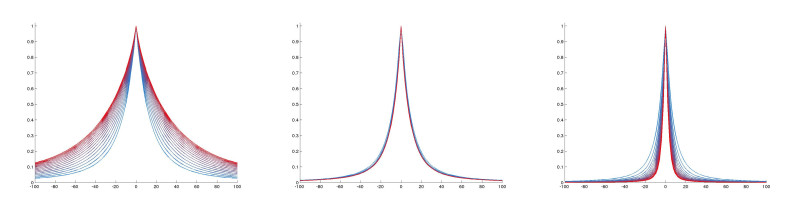
  • Reader Comments
  • © 2021 the Author(s), licensee AIMS Press. This is an open access article distributed under the terms of the Creative Commons Attribution License (http://creativecommons.org/licenses/by/4.0)
通讯作者: 陈斌, bchen63@163.com
  • 1. 

    沈阳化工大学材料科学与工程学院 沈阳 110142

  1. 本站搜索
  2. 百度学术搜索
  3. 万方数据库搜索
  4. CNKI搜索

Metrics

Article views(3447) PDF downloads(595) Cited by(0)

Figures and Tables

Figures(1)

Other Articles By Authors

/

DownLoad:  Full-Size Img  PowerPoint
Return
Return

Catalog