Avocado/Soybean Unsaponifiables (Piacledine&amp;reg;300) show beneficial effect on the metabolism of osteoarthritic cartilage, synovium and subchondral bone: An overview of the mechanisms

Yves Edgard Henrotin; Yves Edgard Henrotin

doi:10.3934/medsci.2018.1.33

AIMS Medical Science

2018, Volume 5, Issue 1: 33-52. doi: 10.3934/medsci.2018.1.33

Previous Article Next Article

Review

Avocado/Soybean Unsaponifiables (Piacledine®300) show beneficial effect on the metabolism of osteoarthritic cartilage, synovium and subchondral bone: An overview of the mechanisms

Yves Edgard Henrotin ^,

Bone and Cartilage Research Unit, Institute of Pathology, Level 5, Arthropôle Liège, University of Liège, CHU Sart-Tilman, 4000 Liège Belgium

Received: 02 September 2017 Accepted: 11 December 2017 Published: 26 December 2017

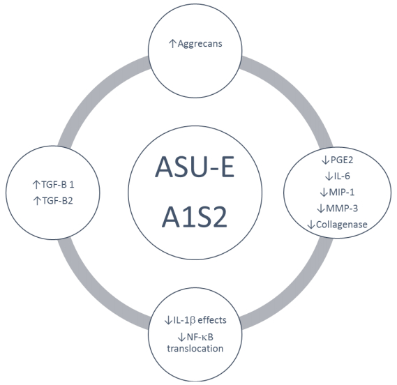
Objectives: The aim of this narrative review of the literature was to synthesize and comment the mechanisms of action of avocado/soybean unsaponifiable mixture (ASU-E, Piascledine®300) on articular tissues involved in the OA pathogenesis. Materials and methods: The search was performed in Pubmed and Scopus between January 1981 and December 2016. Keywords used were—any field—(Cartilage OR Bone OR Synovium) AND Avocado AND Soybean. 32 articles out-off 35 found have been considered. The review has included eleven in vitro and animal studies investigating Avocado Soybean Unsaponifiables (ASU) from Laboratoires Expanscience (Piascledine®300) used separately or in combination. Only research articles published in English and French have been taken into account. Results: ASU-E stimulated proteoglycans synthesis in chondrocytes cultures and counteracted the effects of IL-1 on metalloproteases and inflammatory mediators. Some of these effects were associated with inhibition of NF-kB nuclear translocation and stimulation of TGF-synthesis. ASU-E also positively modulated the altered phenotype of OA subchondral bone osteoblasts and reduced the production of collagenases by synovial cells. Conclusions: ASU-E has positive effects on the metabolic changes of synovium, subchondral bone and cartilage which are the main tissues involved in the pathophysiology of OA. These findings contribute to explain the beneficial effects of ASU-E in clinical trials.
- cartilage,
- bone,
- synovium,
- osteoarthritis,
- avocado,
- soybean
Citation: Yves Edgard Henrotin. Avocado/Soybean Unsaponifiables (Piacledine®300) show beneficial effect on the metabolism of osteoarthritic cartilage, synovium and subchondral bone: An overview of the mechanisms[J]. AIMS Medical Science, 2018, 5(1): 33-52. doi: 10.3934/medsci.2018.1.33

Related Papers:

Abstract

Objectives: The aim of this narrative review of the literature was to synthesize and comment the mechanisms of action of avocado/soybean unsaponifiable mixture (ASU-E, Piascledine®300) on articular tissues involved in the OA pathogenesis. Materials and methods: The search was performed in Pubmed and Scopus between January 1981 and December 2016. Keywords used were—any field—(Cartilage OR Bone OR Synovium) AND Avocado AND Soybean. 32 articles out-off 35 found have been considered. The review has included eleven in vitro and animal studies investigating Avocado Soybean Unsaponifiables (ASU) from Laboratoires Expanscience (Piascledine®300) used separately or in combination. Only research articles published in English and French have been taken into account. Results: ASU-E stimulated proteoglycans synthesis in chondrocytes cultures and counteracted the effects of IL-1 on metalloproteases and inflammatory mediators. Some of these effects were associated with inhibition of NF-kB nuclear translocation and stimulation of TGF-synthesis. ASU-E also positively modulated the altered phenotype of OA subchondral bone osteoblasts and reduced the production of collagenases by synovial cells. Conclusions: ASU-E has positive effects on the metabolic changes of synovium, subchondral bone and cartilage which are the main tissues involved in the pathophysiology of OA. These findings contribute to explain the beneficial effects of ASU-E in clinical trials.

References

[1]	Kraus V, Blanco F, Englund M, et al. (2015) Call for standardized definitions of osteoarthritis and risk stratification for clinical trials and clinical use. Osteoarthr Cartil 23: 1233–1241. doi: 10.1016/j.joca.2015.03.036
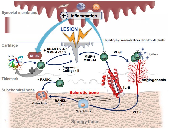
[2]	Pesesse L, Sanchez C, Delcour JP, et al. (2013) Consequences of chondrocyte hypertrophy on osteoarthritic cartilage: potential effect on angiogenesis. Osteoarthr Cartil 21: 1913–1923. doi: 10.1016/j.joca.2013.08.018
[3]	Berenbaum F (2013) Osteoarthritis as an inflammatory disease (osteoarthritis is not osteoarthrosis!). Osteoarthr Cartil 21: 16–21. doi: 10.1016/j.joca.2012.11.012
[4]	Henrotin Y, Pesesse L, Lambert C (2014) Targeting the synovial angiogenesis as a novel treatment approach to osteoarthritis. Ther Adv Musculoskeletal Dis 6: 20–34. doi: 10.1177/1759720X13514669
[5]	Henrotin Y, Pesesse L, Sanchez C (2012) Subchondral bone and osteoarthritis: biological and cellular aspects. Osteoporosis Int 23: 47–51.
[6]	Sanchez C, Pesesse L, Gabay O, et al. (2012) Regulation of subchondral bone osteoblast metabolism by cyclic compression. Arthritis Rheumatol 64: 1193–1203. doi: 10.1002/art.33445
[7]	Sanchez C, Deberg M, Bellahcène A,et al. (2008) Phenotypic characterization of osteoblasts from the sclerotic zones of osteoarthritic subchondral bone. Arthritis Rheumatol 58: 442–455. doi: 10.1002/art.23159
[8]	Pesesse L, Sanchez C, Henrotin Y (2011) Osteochondral plate angiogenesis: a new treatment target in osteoarthritis. Jt Bone Spine 78: 144–149. doi: 10.1016/j.jbspin.2010.07.001
[9]	Rahmati M, Mobasheri A (2016) Mozafari M^.Inflammatory mediators in osteoarthritis: A critical review of the state-of-the-art, current prospects, and future challenges. Bone 85: 81–90.
[10]	Bertuglia A, Lacourt M, Girard C, et al. (2016) Osteoclasts are recruited to the subchondral bone in naturally occurring post-traumatic equine carpal osteoarthritis and may contribute to cartilage degradation. Osteoarthr Cartilage 24: 555–566. doi: 10.1016/j.joca.2015.10.008
[11]	Sanchez C, Gabay O, Salvat C, et al. (2009) Mechanical loading highly increases IL-6 production and decreases OPG expression by osteoblasts. Osteoarthritis Cartilage 7: 473–481.
[12]	Henrotin Y, Pesesse L, Sanchez C (2009) Subchondral bone in osteoarthritis physiopathology: state-of-the art and perspectives. Biomed Mater Eng 19: 311–316.
[13]	Hügle T, Geurts J (2017) What drives osteoarthritis?-synovial versus subchondral bone pathology. Rheumatology (Oxford) 56: 1461–1471.
[14]	Veronese N, Trevisan C, De Rui M, et al. (2015) Osteoarthritis increases the risk of cardiovascular diseases in the elderly: The progetto veneto anziano study. Arthritis Rheumatol 68: 1136–1144.
[15]	Eymard F, Parsons C, Edwards MH, et al. (2015) Diabetes is a risk factor for knee osteoarthritis progression. Osteoarthr Cartilage 23: 851–859. doi: 10.1016/j.joca.2015.01.013
[16]	da Costa BR, Reichenbach S, Keller N, et, al. (2017) Effectiveness of non-steroidal anti-inflammatory drugs for the treatment of pain in knee and hip osteoarthritis: a network meta-analysis. Lancet 387: 2093–2105.
[17]	Roberts E, Delgado Nunes V, Buckner S, et al. (2016) Paracetamol: not as safe as we thought? A systematic literature review of observational studies. Ann Rheum Dis 75: 552–559.
[18]	Pavelka K, Coste P, Géher P, et al. (2010) Efficacy and safety of Piascledine 300 versus chondroitin sulfate in a 6 months treatment plus 2 months observation in patients with osteoarthritis of the knee. Clin Rheumatol 29: 659–670. doi: 10.1007/s10067-010-1384-8
[19]	Appelboom T, Schuermans J, Verbruggen G, et al. (2001) Symptoms modifying effect of avocado/soybean unsaponifiables (ASU) in knee osteoarthritis. A double blind, prospective, placebo-controlled study. Acta Rheumatol Scand 30: 242–247.
[20]	Maheu E, Mazières B, Valat JP, et al. (1998) Symptomatic efficacy of avocado/soybean unsaponifiables in the treatment of osteoarthritis of the knee and hip: a prospective, randomized, double-blind, placebo-controlled, multicenter clinical trial with a six-month treatment period and a two-month followup demonstrating a persistent effect. Arthritis Rheumatol 41: 81–91. doi: 10.1002/1529-0131(199801)41:1<81::AID-ART11>3.0.CO;2-9
[21]	Blotman F, Maheu E, Wulwik A, et al. (1997) Efﬁcacy and safety of avocado/soybean unsaponiﬁables in the treatment of symptomatic osteoarthritis of the knee and hip. A prospective, multicenter, three-month, randomized, double-blind, placebo-controlled trial. Rev Rhum Engl Ed 64: 825–834.
[22]	Christensen R, Bartels EM, Astrup A, et al. (2008) Symptomatic efficacy of avocado-soybean unsaponifiables (ASU) in osteoarthritis (OA) patients: a meta-analysis of randomized controlled trials. Osteoarthritis Cartilage 16: 399–408. doi: 10.1016/j.joca.2007.10.003
[23]	Maheu E, Cadet C, Marty M, et al. (2014) Randomised, controlled trial of avocado-soybean unsaponifiable (Piascledine) effect on structure modification in hip osteoarthritis: the ERADIAS study. Ann Rheum Dis 73: 376–384. doi: 10.1136/annrheumdis-2012-202485
[24]	Zhang W, Doherty M, Arden N, et al. (2005) EULAR evidence based recommendations for the management of hip osteoarthritis: report of a task force of the EULAR Standing Committee for International Clinical Studies Including Therapeutics (ESCISIT). Ann Rheum Dis 64: 669–681. doi: 10.1136/ard.2004.028886
[25]	McAlindon T, Bannuru R, Sullivan M, et al. (2014) OARSI guidelines for the non-surgical management of knee osteoarthritis. Osteoarthr Cartilage 22: 363–388. doi: 10.1016/j.joca.2014.01.003
[26]	Msika P, Baudoin C, Saunois A, et al. (2008) Avocado/Soybean unsaponifiable, ASU EXPANSCIENCE^TM, are strictly different from the nutraceutical products claiming ASU appellation. Osteoarthr Cartilage 16: 1275–1276. doi: 10.1016/j.joca.2008.02.017
[27]	Henrotin Y (2008) Avocado/soybean unsaponifiable (ASU) to treat osteoarthritis: a clarification. Osteoarthritis Cartilage 16: 1118–1119. doi: 10.1016/j.joca.2008.01.010
[28]	Rancurel A (1985) Parfums, cosmétiques, Arômes 61: 91.
[29]	Farines M, Soulier J, Rancurel A, et al. (1995) Influence of avocado oil processing on the nature of some unsaponifiable constituents. J Am Oil Chem Soc 72: 473–476. doi: 10.1007/BF02636092
[30]	Baillet A (1995) Pharmaceutical expert report. Courbevoie, France: Pharmascience, 1995 (unpublished data).
[31]	Mauviel A, Daireaux M, Hartman DJ, et al. (1989) Effets des insaponifiables d'avocat/soja (PIAS) sur la production de collagène par des cultures de synoviocytes, chondrocytes articulaires et fibroblastes dermiques. Rev Rhum 56: 207–213.
[32]	Mauviel A, Loyau G, Pujol JP (1991) Effets des insaponifiables d'avocat/soja (Piascledine) sur l'activité collagénolytique de cultures de synoviocytes rhumatoides humains et de chondrocytes articulaires de lapin traités par l'interleukine-1. Rev Rhum 58: 241–248.
[33]	Harmand MF (1985) Etude de fraction des insaponifiables d'avocat et de soja sur les cultures de chondrocytes articulaires. Gaz Med Fr 92: 1–3.
[34]	Henrotin Y, Labasse A, Jaspar JM, et al. (1998) Effects of three avocado/soybean unsaponifiable mixtures on metalloproteinases, cytokines and prostaglandin E2 production by human articular chondrocytes. Clin. Rheumatol 17: 31–39. doi: 10.1007/BF01450955
[35]	Henrotin Y, Sanchez C, Deberg MA, et al. (2003) Avocado/soybean unsaponifiables increase aggrecan synthesis and reduce catabolic and proinflammatory mediator production by human osteoarthritic chondrocytes. J. Rheumatol 30: 1825–1834
[36]	Gabay O, Gosset M, Levy A, et al. (2008) Stress-induced signaling pathways in hyalin chondrocytes: inhibition by Avocado-Soybean Unsaponifiables (ASU). Osteoarthr Cartilage 16: 373–384. doi: 10.1016/j.joca.2007.06.016
[37]	Boumediene K, Felisaz N, Bogdanowicz P, et al. (1999) Avocado/soya unsaponifiables enhance the expression of transforming growth factor beta1 and beta2 in cultured articular chondrocytes. Arthritis Rheumatol 42: 148–156. doi: 10.1002/1529-0131(199901)42:1<148::AID-ANR18>3.0.CO;2-U
[38]	Campbell IK, Wojta J, Novak U, et al. (1994) Cytokine modulation of plasminogen activator inhibitor-1 (PAI-1) production by human articular cartilage and chondrocytes: down-regulation by tumor necrosis factora. Biochim Biophys Acta 1226: 277–285. doi: 10.1016/0925-4439(94)90038-8
[39]	Khayyal MT, el-Ghazaly MA (1998) The possible "chondroprotective" effect of the unsaponifiable constituents of avocado and soya in vivo. Drugs Exp Clin Res 24: 41–50.
[40]	Boileau C, Martel-Pelletier J, Caron J, et al. (2009) Protective effects of total fraction of avocado/soybean unsaponifiables on the structural changes in experimental dog osteoarthritis: inhibition of nitric oxide synthase and matrix metalloproteinase-13. Arthritis Res Ther 11: 41. doi: 10.1186/ar2649
[41]	Jaberi, F, Tahami, M, Torabinezhad S, et al. (2012) The healing effect of soybean and avocado mixture on knee cartilage defects in a dog animal model. Comp. Clin Pathol 21: 661–666. doi: 10.1007/s00580-010-1152-9
[42]	Altinel L, Saritas ZK, Kose KC, et al. (2007) Treatment with unsaponifiable extracts of avocado and soybean increases TGF-beta1 and TGF-beta2 levels in canine joint fluid. Tohoku J Exp Med 211: 181–186. doi: 10.1620/tjem.211.181
[43]	Cake M, Read R, Guillou B, et al. (2008) Modification of articular cartilage and subchondral bone pathology in an ovine meniscectomy model of osteoarthritis by avocado and soya unsaponifiables (ASU). Osteoarthr Cartilage 8: 404–411.
[44]	Cinelli M, Guiducci S, Del Rosso A, et al. (2006) Piascledine modulates the production of VEGF and TIMP-1 and reduces the invasiveness of rheumatoid arthritis synoviocytes. Scand J Rheumatol 35: 346–350. doi: 10.1080/03009740600709865
[45]	Henrotin Y, Deberg M, Crielaard JM, et al. (2006) Avocado/soybean unsaponifiables prevent the inhibitory effect of osteoarthritic subchondral osteoblasts on aggrecan and type II collagen synthesis by chondrocytes. J Rheumatol 33: 1668–1678.
[46]	Sanchez C, Deberg M, Piccardi N, et al. (2005) Osteoblasts from the sclerotic subchondral bone downregulate aggrecan but upregulate metalloproteinases expression by chondrocytes. This effect is mimicked by interleukin-6, -1beta and oncostatin M pre-treated non-sclerotic osteoblasts. Osteoarthr Cartilage 13: 979–987.
[47]	Sanchez C, Deberg M, Piccardi N, et al. (2004) Interleukin-1, interleukin-6 and oncostatin M stimulate normal subchondral osteoblast to induce cartilage degradation. Osteoarthr Cart 12: S98.
[48]	Andriamanalijaona R, Benateau H, Barre PE, et al. (2006) Effect of interleukin-1beta on transforming growth factor-beta and bone morphogenetic protein-2 expression in human periodontal ligament and alveolar bone cells in culture: modulation by avocado and soybean unsaponifiables. J Periodontol 77: 1156–1166. doi: 10.1902/jop.2006.050356
[49]	Day JS, van der Linden JC, Bank RA, et al. (2004) Adaptation of subchondral bone in osteoarthritis. Biorheology 41: 359–368.
[50]	Westacott CI, Webb GR, Warnock MG, et al. (1997) Alteration of cartilage metabolism by cells from osteoarthritic bone. Arthritis Rheumatol 40: 1282–1291. doi: 10.1002/1529-0131(199707)40:7<1282::AID-ART13>3.0.CO;2-E
[51]	Hilal G, Massicotte F, Martel-Pelletier J, et al. (2001) Endogenous prostaglandin E2 and insulin-like growth factor 1 can modulate the levels of parathyroid hormone receptor in human osteoarthritic osteoblasts. J Bone Miner Res 16: 713–721. doi: 10.1359/jbmr.2001.16.4.713
[52]	Hilal G, Martel-Pelletier J, Pelletier JP, et al. (1999) Abnormal regulation of urokinase plasminogen activator by insulin-like growth factor 1 in human osteoarthritic subchondral osteoblasts. Arthritis Rheumatol 42: 2112–2122. doi: 10.1002/1529-0131(199910)42:10<2112::AID-ANR11>3.0.CO;2-N
[53]	Massicotte F, Fernandes JC, Martel-Pelletier J, et al. (2006) Modulation of insulin-like growth factor 1 levels in human osteoarthritic subchondral bone osteoblasts. Bone 38: 333–341. doi: 10.1016/j.bone.2005.09.007
[54]	Hilal G, Martel-Pelletier J, Pelletier JP, et al. (1998) Osteoblast-like cells from human subchondral osteoarthritic bone demonstrate an altered phenotype in vitro: possible role in subchondral bone sclerosis. Arthritis Rheumatol 41: 891–899. doi: 10.1002/1529-0131(199805)41:5<891::AID-ART17>3.0.CO;2-X
[55]	Harris SE, Bonewald LF, Harris MA, et al. (1994) Effects of transforming growth factor on bone nodule formation and expression of bone morphogenetic protein 2, osteocalcin, osteopontin, alkaline phosphatase, and type I collagen mRNA in long-term cultures of fetal rat calvarial osteoblasts. J Bone Miner Res 9: 855–863.

Reader Comments

Your name:*

Email:*
© 2018 the Author(s), licensee AIMS Press. This is an open access article distributed under the terms of the Creative Commons Attribution License (http://creativecommons.org/licenses/by/4.0)