A two-group epidemic model with heterogeneity in cognitive effects

Zehan Liu; Daoxin Qiu; Shengqiang Liu; Zehan Liu; Daoxin Qiu; Shengqiang Liu

doi:10.3934/mbe.2025040

Mathematical Biosciences and Engineering

2025, Volume 22, Issue 5: 1109-1139. doi: 10.3934/mbe.2025040

Previous Article Next Article

Research article Special Issues

A two-group epidemic model with heterogeneity in cognitive effects

School of Mathematical Sciences, Tiangong University, Tianjin 300387, China

Received: 20 February 2025 Revised: 16 March 2025 Accepted: 21 March 2025 Published: 08 April 2025

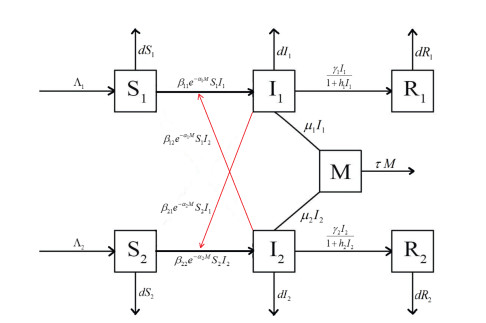
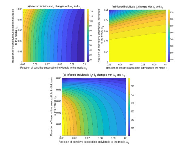
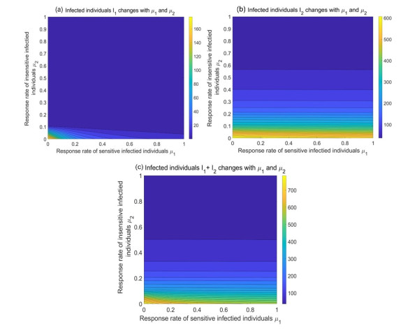
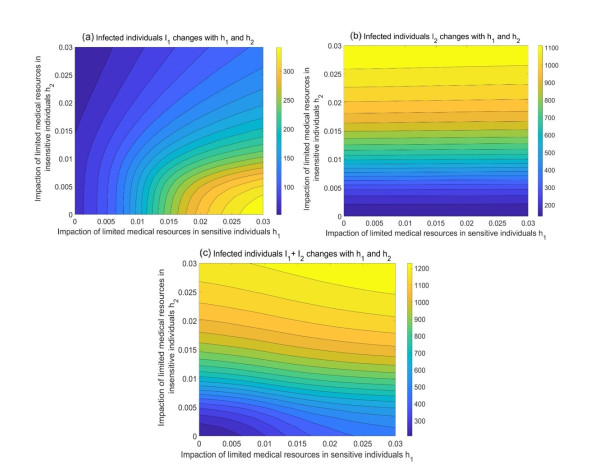
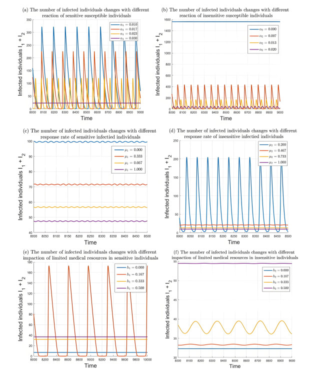
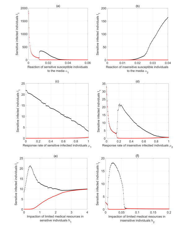
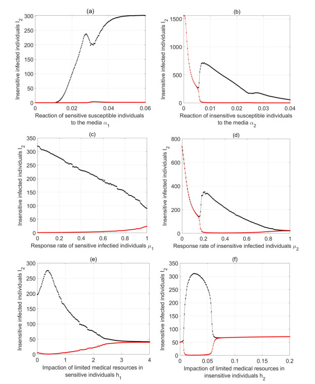
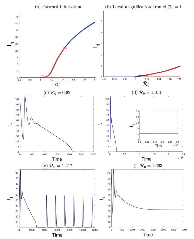
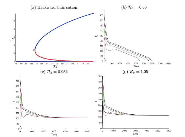
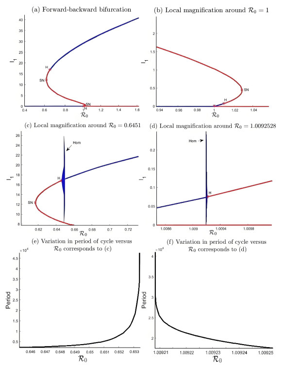
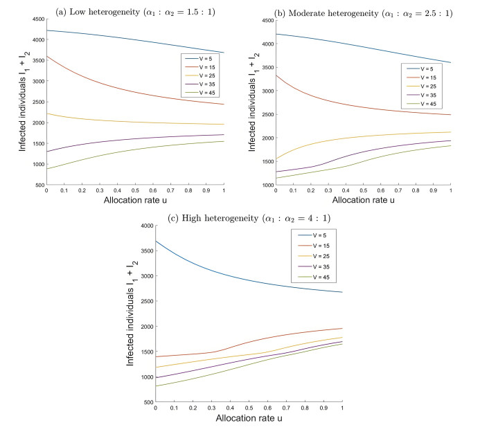
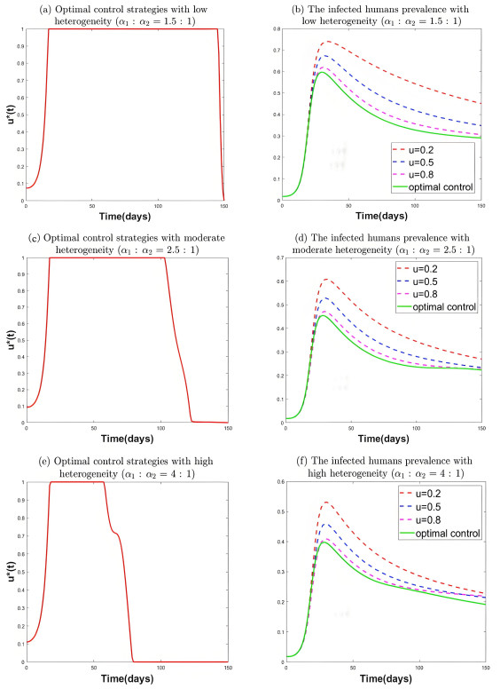
During the outbreak of new infectious diseases, media information and medical resources play crucial roles in shaping the dynamics of disease transmission. To investigate the combined impact of media information and limited medical resources on disease spread, we proposed a two-group compartmental model. This model divided the population into two groups based on their ability to receive information. We derived the basic reproduction number, analyzed the local stability of the disease-free equilibrium, and examined the conditions under which disease extinction or persistence occured. For control strategies, we explored both constant and optimal control approaches under the constraint of limited media resources. Numerical simulations indicated that enhancing the population's responsiveness to media and medical resources helped reduce the infection rate. The model also exhibited complex dynamical behaviors, such as backward bifurcation, forward-backward bifurcation, and homoclinic bifurcation, which presented significant challenges for disease control. Furthermore, we conducted numerical simulations of the optimal control problem to validate and support our theoretical findings. In the case of constant control, as the disparity between the two populations increases, media resources should be increasingly allocated to the information-insensitive group. For optimal control, we employed the forward-backward sweep method, where media resources were increasingly allocated to information-insensitive groups as population heterogeneity rises. This study established an empirical framework for optimizing media-driven public health communication strategies, offering critical insights into the strategic allocation of limited media resources across heterogeneous populations.
- two-group compartment model,
- heterogeneous,
- media information,
- limited medical resources,
- control strategies,
- bifurcation
Citation: Zehan Liu, Daoxin Qiu, Shengqiang Liu. A two-group epidemic model with heterogeneity in cognitive effects[J]. Mathematical Biosciences and Engineering, 2025, 22(5): 1109-1139. doi: 10.3934/mbe.2025040

Related Papers:

Abstract

During the outbreak of new infectious diseases, media information and medical resources play crucial roles in shaping the dynamics of disease transmission. To investigate the combined impact of media information and limited medical resources on disease spread, we proposed a two-group compartmental model. This model divided the population into two groups based on their ability to receive information. We derived the basic reproduction number, analyzed the local stability of the disease-free equilibrium, and examined the conditions under which disease extinction or persistence occured. For control strategies, we explored both constant and optimal control approaches under the constraint of limited media resources. Numerical simulations indicated that enhancing the population's responsiveness to media and medical resources helped reduce the infection rate. The model also exhibited complex dynamical behaviors, such as backward bifurcation, forward-backward bifurcation, and homoclinic bifurcation, which presented significant challenges for disease control. Furthermore, we conducted numerical simulations of the optimal control problem to validate and support our theoretical findings. In the case of constant control, as the disparity between the two populations increases, media resources should be increasingly allocated to the information-insensitive group. For optimal control, we employed the forward-backward sweep method, where media resources were increasingly allocated to information-insensitive groups as population heterogeneity rises. This study established an empirical framework for optimizing media-driven public health communication strategies, offering critical insights into the strategic allocation of limited media resources across heterogeneous populations.

References

[1]	M. Benzeval, C. L. Booker, J. Burton, T. F. Crossley, A. Jackle, M. Kumari, et al., Briefing Note COVID-19 Survey: Health and Caring, Understanding Society Working Paper Series, 2020.
[2]	F. S. Dawood, S. Jain, L. Finelli, M. W. Shaw, S. Lindstrom, R. J. Garten, et al., Emergence of a novel swine-origin influenza a (H1N1) virus in humans, N. Eng. J. Med., 360 (2009), 2605–2615. https://doi.org/10.1056/NEJMoa0903810 doi: 10.1056/NEJMoa0903810
[3]	R. D. Smith, Responding to global infectious disease outbreaks: Lessons from SARS on the role of risk perception, communication and management, Soc. Sci. Med., 63 (2006), 3113–3123. https://doi.org/10.1016/j.socscimed.2006.08.004 doi: 10.1016/j.socscimed.2006.08.004
[4]	W. Kawohl, C. Nordt, COVID-19, unemployment, and suicide, Lancet Psychiatry, 7 (2020), 389–390. https://doi.org/10.1016/S2215-0366(20)30141-3 doi: 10.1016/S2215-0366(20)30141-3
[5]	W. W. Thompson, D. K. Shay, E. Weintraub, L. Brammer, N. Cox, L. J. Anderson, et al., Mortality associated with influenza and respiratory syncytial virus in the United States, J. Am. Med. Assoc., 289 (2003), 179–186. https://doi.org/10.1001/jama.289.2.179 doi: 10.1001/jama.289.2.179
[6]	H. Li, L. Pan, W. Chen, The influence of media information sources on preventive behaviors in China: After the outbreak of COVID-19 pandemic, Math. Method. Appl. Sci., 42 (2023). https://doi.org/10.1155/2023/4941436 doi: 10.1155/2023/4941436
[7]	G. Qian, M. Ada, N. Yang, A COVID-19 transmission within a family cluster by presymptomatic infectors in China, Clin. Infect. Dis., 71 (2020), 15. https://doi.org/10.1093/cid/ciaa316 doi: 10.1093/cid/ciaa316
[8]	Z. Niu, Z. Qin, P. Hu, T. Wang, Health beliefs, trust in media sources, health literacy, and preventive behaviors among high-risk Chinese for COVID-19, Health Promot. Int., 37 (2022), 1004–1012. https://doi.org/10.1080/10410236.2021.1880684 doi: 10.1080/10410236.2021.1880684
[9]	A. Wang, Y. Xiao, A Filippov system describing media effects on the spread of infectious diseases, Nonlinear Anal. Hybri., 11 (2013), 84–97. https://doi.org/10.1016/j.nahs.2013.06.005 doi: 10.1016/j.nahs.2013.06.005
[10]	M. L. Diagne, F. B. Agusto, H. Rwezaura, J. M. Tchuenche, S. Lenhart, Optimal control of an epidemic model with treatment in the presence of media coverage, Sci. Afr., 24 (2024), e02138. https://doi.org/10.1016/j.sciaf.2024.e02138 doi: 10.1016/j.sciaf.2024.e02138
[11]	Y. Xiao, S. Tang, J. Wu, Media impact switching surface during an infectious disease outbreak, Sci. Rep., 5 (2015), 7838. https://doi.org/10.1038/srep07838 doi: 10.1038/srep07838
[12]	J. Xie, H. Guo, M. Zhang, Dynamics of an SEIR model with media coverage mediated nonlinear infectious force. Math. Biosci. Eng., 20 (2023), 14616–14633. https://doi.org/10.3934/mbe.2023654 doi: 10.3934/mbe.2023654
[13]	W. Zhou, Y. Xiao, J. M. Heffernan, Optimal media reporting intensity on mitigating spread of an emerging infectious disease, PLoS One, 14 (2019), e0213898. https://doi.org/10.1371/journal.pone.0213898 doi: 10.1371/journal.pone.0213898
[14]	L. Hu, L. Nie, Stability and Hopf bifurcation analysis of a multi-delay Vector-Borne disease model with presence awareness and media effect, Fractal Fract., 7 (2023), 831. https://doi.org/10.3390/fractalfract7120831 doi: 10.3390/fractalfract7120831
[15]	K. K. Pal, R. K. Rai, P. K. Tiwari, Impact of psychological fear and media on infectious diseases induced by carriers, Chaos, 34 (2024), 123168. https://doi.org/10.1063/5.0217936 doi: 10.1063/5.0217936
[16]	N. Wang, L. Qi, M. Bessane, M. Hao, Global Hopf bifurcation of a two-delay epidemic model with media coverage and asymptomatic infection, J. Differ. Equations, 369 (2023), 1–40. https://doi.org/10.1016/j.jde.2023.05.036 doi: 10.1016/j.jde.2023.05.036
[17]	Y. Luo, P. Liu, T. Zheng, Z. Teng, Dynamic analysis of an SSvEIQR model with nonlinear contact rate, isolation rate and vaccination rate dependent on media coverage, Int. J. Biomath., (2024), 2450011. https://doi.org/10.1142/S1793524524500116
[18]	H. Zang, S. Liu, Y. Lin, Evaluations of heterogeneous epidemic models with exponential and non-exponential distributions for latent period: The Case of COVID-19, Math. Biosci. Eng., 20 (2023), 12579–12598. https://doi.org/10.3934/mbe.2023560 doi: 10.3934/mbe.2023560
[19]	H. Zang, Y. Lin, S. Liu, Global dynamics of heterogeneous epidemic models with exponential and nonexponential latent period distributions, Stud. Appl. Math., 152 (2024), 1365–1403. https://doi.org/10.1111/sapm.12678 doi: 10.1111/sapm.12678
[20]	Y. Lin, H. Zang, S. Liu, Final size of an $n$-group SEIR epidemic model with nonlinear incidence rate, Int. J. Biomath., 11 (2024). https://doi.org/10.1142/S1793524524500086
[21]	T. Li, Y. Xiao, Linking the disease transmission to information dissemination dynamics: An insight from a multi-scale model study, J. Theor. Biol., 526 (2021), 110796. http://doi.org/10.1016/j.jtbi.2021.110796 doi: 10.1016/j.jtbi.2021.110796
[22]	J. Cui, X. Mu, H. Wan, Saturation recovery leads to multiple endemic equilibria and backward bifurcation, J. Theor. Biol., 254 (2008), 275–283. https://doi.org/10.1016/j.jtbi.2008.05.015 doi: 10.1016/j.jtbi.2008.05.015
[23]	X. Zhou, J. Cui, Analysis of stability and bifurcation for an SEIR epidemic model with saturated recovery rate, Commun. Nonlinear Sci., 16 (2011), 4438–4450. http://dx.doi.org/10.1016/j.cnsns.2011.03.026 doi: 10.1016/j.cnsns.2011.03.026
[24]	X. Wang, J. Li, S. Guo, M. Liu, Dynamic analysis of an Ebola epidemic model incorporating limited medical resources and immunity loss, J. Appl. Math. Comput., 69 (2023), 4229–4242. https://doi.org/10.1007/s12190-023-01923-2 doi: 10.1007/s12190-023-01923-2
[25]	J. K. Asamoah, F. Nyabadza, Z. Jin, E. Bonyah, M. A. Khan, M. Y. Li, et al., Backward bifurcation and sensitivity analysis for bacterial meningitis transmission dynamics with a nonlinear recovery rate, Chaos Solitons Fractals, 140 (2020), 110237. https://doi.org/10.1016/j.chaos.2020.110237 doi: 10.1016/j.chaos.2020.110237
[26]	T. Li, Y. Xiao, Complex dynamics of an epidemic model with saturated media coverage and recovery, Nonlinear Dyn., 107 (2022), 2995–3023. https://doi.org/10.1007/s11071-021-07096-6 doi: 10.1007/s11071-021-07096-6
[27]	Y. Hao, Y. Luo, Z. Teng, Role of limited medical resources in an epidemic model with media report and general birth rate, Infect. Dis. Modell., 10 (2025), 522–535. https://doi.org/10.1016/j.idm.2025.01.001 doi: 10.1016/j.idm.2025.01.001
[28]	P. Dreessche, J. Watmough, Reproduction numbers and sub-threshold endemic equilibria for compartmental models of disease transmission, Math. Biosci., 180 (2002), 29–48. https://doi.org/10.1016/S0025-5564(02)00108-6 doi: 10.1016/S0025-5564(02)00108-6
[29]	J. P. L. Salle, The stability of dynamical systems, in CBMS-NSF Regional Conference Series in Applied Mathematics, (1976). https://doi.org/10.1137/1.9781611970432
[30]	H. Thieme, R. Horst, Persistence under relaxed point-dissipativity (with application to an endemic model), SIAM J. Math. Anal., 24 (2006), 407–435. https://doi.org/10.1137/0524026 doi: 10.1137/0524026
[31]	W. Wang, X. Zhao, An epidemic model in a patchy environment, Math. Biosci., 19 (2004), 97–112. https://doi.org/10.1016/j.mbs.2002.11.001 doi: 10.1016/j.mbs.2002.11.001
[32]	H. L. Smith, X. Zhao, Robust persistence for semidynamical systems, Nonlinear Anal., 47 (2001), 6169–6179. https://doi.org/10.1016/S0362-546X(01)00678-2 doi: 10.1016/S0362-546X(01)00678-2
[33]	M. W. Hirsch, H. L. Smith, X. Zhao, Chain transitivity, attractivity, and strong repellors for semidynamical systems, J. Dyn. Differ. Equations, 13 (2001), 107–131. https://doi.org/10.1023/A:1009044515567 doi: 10.1023/A:1009044515567
[34]	X. Zhao, Uniform persistence and periodic coexistence states in infinite-dimensional periodic semiflows with applications, Can. Appl. Math., 3 (1995), 473–495.
[35]	W. Fleming, R. Rishel, Deterministic and Stochastic Optimal Control, 1st edition, Springer-Verlag, New York, 1975.
[36]	L. S. Pontryagin, V. G. Boltyanskii, R. V. Gamkrelidze, E. F. Mishchenko, The Mathematical Theory of Optimal Processes, Interscience Publishers John Wiley and Sons, Inc., New York-London, 1962.
[37]	H. Zhang, Z. Yang, K. A. Pawelek, S. Liu, Optimal control strategies for a two-group epidemic model with vaccination-resource constraints, Appl. Math. Comput., 371 (2020), 124956. https://doi.org/10.1016/j.amc.2019.124956 doi: 10.1016/j.amc.2019.124956
[38]	Q. Yan, S. Tang, S. Gabriele, J. Wu, Media coverage and hospital notifications: Correlation analysis and optimal media impact duration to manage a pandemic, J. Theor. Biol., 390 (2016), 1–13. https://doi.org/10.1016/j.jtbi.2015.11.002 doi: 10.1016/j.jtbi.2015.11.002
[39]	K. W. Blayneh, A. B. Gumel, S. Lenhart, T. Clayton, Backward bifurcation and optimal control in transmission dynamics of west nile virus, B. Math. Biol., 72 (2010), 1006–1028. https://doi.org/10.1007/s11538-009-9480-0 doi: 10.1007/s11538-009-9480-0

Reader Comments

Your name:*

Email:*
© 2025 the Author(s), licensee AIMS Press. This is an open access article distributed under the terms of the Creative Commons Attribution License (http://creativecommons.org/licenses/by/4.0)