Finite-time stability (FTS) has attained great interest in nonlinear control systems in recent two decades. Fixed-time stability (FxTS) is an improved version of FTS in consideration of its settling time independent of the initial values. In this article, the adaptive fixed-time stabilization issue is studied for a kind of nonlinear systems with nonlinear parametric uncertainties and uncertain control coefficients. Using the adaptive estimate and the adding one power integrator (AOPI) design tool, we propose a two-phase control strategy, which makes that the system states tend to the origin in fixed-time, and other signals are bounded on $ [0, +\infty) $. We prove the main results by means of the recently developed fixed-time Lyapunov stability theory. Finally, we apply the proposed adaptive fixed-time stabilizing control strategy into the pendulum system, and the simulation results verify the efficacy of the presented method.
Citation: Yan Zhao, Jianli Yao, Jie Tian, Jiangbo Yu. Adaptive fixed-time stabilization for a class of nonlinear uncertain systems[J]. Mathematical Biosciences and Engineering, 2023, 20(5): 8241-8260. doi: 10.3934/mbe.2023359
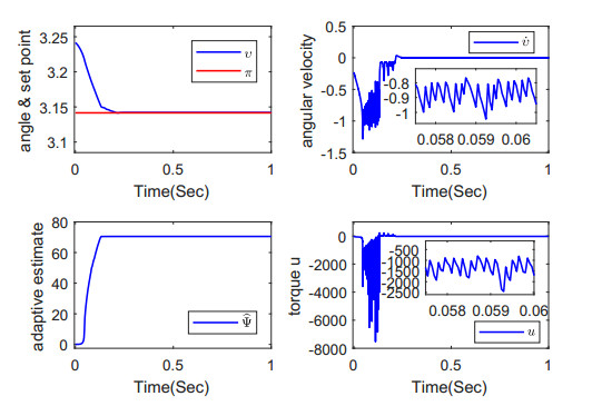
Finite-time stability (FTS) has attained great interest in nonlinear control systems in recent two decades. Fixed-time stability (FxTS) is an improved version of FTS in consideration of its settling time independent of the initial values. In this article, the adaptive fixed-time stabilization issue is studied for a kind of nonlinear systems with nonlinear parametric uncertainties and uncertain control coefficients. Using the adaptive estimate and the adding one power integrator (AOPI) design tool, we propose a two-phase control strategy, which makes that the system states tend to the origin in fixed-time, and other signals are bounded on $ [0, +\infty) $. We prove the main results by means of the recently developed fixed-time Lyapunov stability theory. Finally, we apply the proposed adaptive fixed-time stabilizing control strategy into the pendulum system, and the simulation results verify the efficacy of the presented method.

| [1] | I. Karafyllis, Z. P. Jiang, Stability and Stabilization of Nonlinear Systems, Springer-Verlag, 2011. https://doi.org/10.1007/978-0-85729-513-2 |
| [2] | M. Krsti$\acute{c}$, I. Kanellakopoulos, P. V. Kokotovi$\acute{c}$, Nonlinear and Adaptive Control Design, Wiley, 1995. |
| [3] | M. Athans, P. L. Falb, Optimal Control: An Introduction to Theory and Its Applications, McGraw-Hill, 1966. |
| [4] |
S. P. Bhat, D. S. Bernstein, Continuous finite-time stabilization of the translational and rotational double integrators, IEEE Trans. Auto. Control, 43 (1998), 678–682. https://doi.org/10.1109/9.668834 doi: 10.1109/9.668834

|
| [5] |
Y. Hong, Finite-time stabilization and stabilizability of a class of controllable systems, Syst. Control Lett., 46 (2002), 231–236. https://doi.org/10.1016/S0167-6911(02)00119-6 doi: 10.1016/S0167-6911(02)00119-6
|
| [6] |
Y. Hong, J. Wang, D. Cheng, Adaptive finite-time control of nonlinear systems with parametric uncertainty, IEEE Trans. Auto. Control, 51 (2006), 858-862. https://doi.org/10.1109/TAC.2006.875006 doi: 10.1109/TAC.2006.875006
|
| [7] |
V. T. Haimo, Finite time controllers, SIAM J. Control Optim., 24 (1986), 760–770. https://doi.org/10.1137/0324047 doi: 10.1137/0324047
|
| [8] |
X. Huang, W. Lin, B. Yang, Global finite-time stabilization of a class of uncertain nonlinear systems, Automatica, 41 (2005), 881–888. https://doi.org/10.1016/j.automatica.2004.11.036 doi: 10.1016/j.automatica.2004.11.036
|
| [9] |
X. Y. Yang, X. D. Li, Finite-time stability of nonlinear impulsive systems with applications to neural networks, IEEE Trans. Neural Networks Learning Syst., 34 (2021), 243–251. https://doi.org/10.1109/TNNLS.2021.3093418 doi: 10.1109/TNNLS.2021.3093418
|
| [10] |
X. D. Li, X. Y. Yang, S. J. Song, Lyapunov conditions for finite-time stability of time-varying time-delay systems, Automatica, 103 (2019), 135–140. https://doi.org/10.1016/j.automatica.2019.01.031 doi: 10.1016/j.automatica.2019.01.031
|
| [11] |
X. D. Li, D. W. C. Ho, J. D. Cao, Finite-time stability and settling-time estimation of nonlinear impulsive systems, Automatica, 99 (2019), 361–368. https://doi.org/10.1016/j.automatica.2018.10.024 doi: 10.1016/j.automatica.2018.10.024
|
| [12] |
J. Fu, R. Ma, T. Chai, Global finite-time stabilization of a class of switched nonlinear systems with the powers of positive odd rational numbers, Automatica, 54 (2015), 360–373. https://doi.org/10.1016/j.automatica.2015.02.023 doi: 10.1016/j.automatica.2015.02.023
|
| [13] |
Y. G. Liu, Global finite-time stabilization via time-varying feedback for uncertain nonlinear systems, SIAM J. Control Optim., 52 (2014), 1886–1913. https://doi.org/10.1137/130920423 doi: 10.1137/130920423
|
| [14] |
F. Z. Li, Y. G. Liu, Global finite-time stabilization via time-varying output-feedback for uncertain nonlinear systems with unknown growth rate, Int. J. Robust Nonlinear Control, 27 (2017), 4050–4070. https://doi.org/10.1002/rnc.3743 doi: 10.1002/rnc.3743
|
| [15] |
J. Huang, C. Wen, W. Wang, Y. Song, Design of adaptive finite-time controllers for nonlinear uncertain systems based on given transient specifications, Automatica, 69 (2016), 395–404. https://doi.org/10.1016/j.automatica.2015.08.013 doi: 10.1016/j.automatica.2015.08.013
|
| [16] |
S. P. Huang, Z. R. Xiang, Finite-time stabilization of switched stochastic nonlinear systems with mixed odd and even powers, Automatica, 73 (2016), 130–137. https://doi.org/10.1016/j.automatica.2016.06.023 doi: 10.1016/j.automatica.2016.06.023
|
| [17] |
S. H. Ding, S. H. Li, Second-order sliding mode controller design subject to mismatched term, Automatica, 77 (2017), 388–392. https://doi.org/10.1016/j.automatica.2016.07.038 doi: 10.1016/j.automatica.2016.07.038
|
| [18] |
H. B. Du, C. J. Qian, S. Z. Yang, S. H. Li, Recursive design of finite-time convergent observers for a class of time-varying nonlinear systems, Automatica, 49 (2013), 601–609. https://doi.org/10.1016/j.automatica.2012.11.036 doi: 10.1016/j.automatica.2012.11.036
|
| [19] |
Z. Y. Sun, Y. Shao, C.C. Chen, Fast finite-time stability and its application in adaptive control of high-order nonlinear system, Automatica, 106 (2019), 339–348. https://doi.org/10.1016/j.automatica.2019.05.018 doi: 10.1016/j.automatica.2019.05.018
|
| [20] |
C. C. Chen, Z.Y. Sun, A unified approach to finite-time stabilization of high-order nonlinear systems with an asymmetric output constraint, Automatica, 111 (2020), 108581. https://doi.org/10.1016/j.automatica.2019.108581 doi: 10.1016/j.automatica.2019.108581
|
| [21] |
Z. Y. Li, J. Y. Zhai, H.R. Karimi, Adaptive finite-time super-twisting sliding mode control for robotic manipulators with control backlash, Int. J. Robust Nonlinear Control, 31 (2021), 8537–8550. https://doi.org/10.1002/rnc.5744 doi: 10.1002/rnc.5744
|
| [22] |
M. M. Jiang, X. J. Xie, Adaptive finite-time stabilisation of high-order uncertain nonlinear systems, Int. J. Control, 91 (2018), 2159–2169. https://doi.org/10.1080/00207179.2016.1245869 doi: 10.1080/00207179.2016.1245869
|
| [23] |
A. Polyakov, Nonlinear feedback design for fixed-time stabilization of linear control systems, IEEE Trans. Automatic Control, 57 (2012), 2106–2110. https://doi.org/10.1109/TAC.2011.2179869 doi: 10.1109/TAC.2011.2179869
|
| [24] |
V. Andrieu, L. Praly, A. Astolfi, Homogeneous approximation, recursive observer design, and output feedback, SIAM J. Control Optim., 47 (2008), 1814–1850. https://doi.org/10.1137/060675861 doi: 10.1137/060675861
|
| [25] |
A. Polyakov, D. Efimov, W. Perruquetti, Finite-time and fixed-time stabilization: Implicit Lyapunov function approach, Automatica, 51 (2015), 332–340. https://doi.org/10.1016/j.automatica.2014.10.082 doi: 10.1016/j.automatica.2014.10.082
|
| [26] |
F. Lopez-Ramirez, A. Polyakov, D. Efimov, W. Perruquetti, Finite-time and fixed-time observer design: Implicit Lyapunov function approach, Automatica, 87 (2018), 52–60. https://doi.org/10.1016/j.automatica.2017.09.007 doi: 10.1016/j.automatica.2017.09.007
|
| [27] |
Z. Y. Zuo, Nonsingular fixed-time terminal sliding mode control of non-linear systems, IET Control Theory Appl., 9 (2014), 545–552. https://doi.org/10.1049/iet-cta.2014.0202 doi: 10.1049/iet-cta.2014.0202
|
| [28] |
C. Hua, Y. Li, X. Guan, Finite/Fixed-time stabilization for nonlinear interconnected systems with dead-zone input, IEEE Trans. Auto. Control, 62 (2017), 2554–2560. https://doi.org/10.1109/TAC.2016.2600343 doi: 10.1109/TAC.2016.2600343
|
| [29] |
Z. Y. Zuo, B. L. Tian, M. Defoort, Z. T. Ding, Fixed-time consensus tracking for multi-agent systems with high-order integrator dynamics, IEEE Trans. Auto. Control, 63 (2018), 563–570. https://doi.org/10.1109/TAC.2017.2729502 doi: 10.1109/TAC.2017.2729502
|
| [30] |
Z. C. Liang, Z. N. Wang, J. Zhao, P. K. Wong, Z. X. Yang, Z. T. Ding, Fixed-time and fault-tolerant path following control for autonomous vehicles with unknown parameters subject to prescribed performance, IEEE Trans. Syst. Man Cybern. Syst., 2022 (2022), 1–11. https://doi.org/10.1109/TSMC.2022.3211624 doi: 10.1109/TSMC.2022.3211624
|
| [31] |
Z. C. Liang, Z. N. Wang, J. Zhao, P. K. Wong, Z. X. Yang, Z. T. Ding, Fixed-time prescribed performance path-following control for autonomous vehicle with complete unknown parameters, IEEE Trans. Ind. Electron., 2022 (2022), 1–10. https://doi.org/10.1109/TIE.2022.3210544 doi: 10.1109/TIE.2022.3210544
|
| [32] |
J. B. Yu, A. Stancu, Z. T. Ding, Y. Q. Wu, Adaptive finite/fixed-time stabilizing control for nonlinear systems with parametric uncertainty, Int. J. Robust Nonlinear Control, 33 (2023), 1513–1530. https://doi.org/10.1002/rnc.6441 doi: 10.1002/rnc.6441
|
| [33] |
Z. C. Zhang, Y. Q. Wu, Fixed-time regulation control of uncertain nonholonomic systems and its applications, Int. J. Control, 90 (2017), 1327–1344. https://doi.org/10.1080/00207179.2016.1205758 doi: 10.1080/00207179.2016.1205758
|
| [34] |
C. Y. Wang, H. Tnunay, Z. Y. Zuo, B. Lennox, Z. T. Ding, Fixed-time formation control of multirobot systems: design and experiments, IEEE Trans. Ind. Electron., 66 (2019), 6292–6301. https://doi.org/10.1109/TIE.2018.2870409 doi: 10.1109/TIE.2018.2870409
|
| [35] |
J. B. Yu, Y. Zhao, Y. Q. Wu, Global robust output tracking control for a class of uncertain cascaded nonlinear systems, Automatica, 93 (2018), 274–281. https://doi.org/10.1016/j.automatica.2018.03.018 doi: 10.1016/j.automatica.2018.03.018
|
| [36] |
Z. G. Liu, Y. Q. Wu, Universal strategies to explicit adaptive control of nonlinear time-delay systems with different structures, Automatica, 89 (2018), 151–159. https://doi.org/10.1016/j.automatica.2017.11.023 doi: 10.1016/j.automatica.2017.11.023
|
| [37] |
Q. Guo, Z. Y. Zuo, Z. T. Ding, Parametric adaptive control of single-rod electrohydraulic system with block-strict-feedback model, Automatica, 113 (2020), 108807. https://doi.org/10.1016/j.automatica.2020.108807 doi: 10.1016/j.automatica.2020.108807
|
| [38] |
M. Basin, C. B. Panathula, Y. Shtessel, Adaptive uniform finite/fixed-time convergent second-order sliding-mode control, Int. J. Control, 89 (2016), 1777–1787. https://doi.org/10.1080/00207179.2016.1184759 doi: 10.1080/00207179.2016.1184759
|
| [39] |
Z. W. Zheng, M. Feroskhan, L. Sun, Adaptive fixed-time trajectory tracking control of a stratospheric airship, ISA Trans., 76 (2018), 134–144. https://doi.org/10.1016/j.isatra.2018.03.016 doi: 10.1016/j.isatra.2018.03.016
|
| [40] |
Y. Huang, Y. M. Jia, Adaptive fixed-time six-DOF tracking control for noncooperative spacecraft fly-around mission, IEEE Trans. Control Syst. Technol., 27 (2019), 1796–1804. https://doi.org/10.1109/TCST.2018.2812758 doi: 10.1109/TCST.2018.2812758
|
| [41] |
Q. Chen, S. Z. Xie, M. X. Sun, X. X. He, Adaptive nonsingular fixed-Time attitude stabilization of uncertain spacecraft, IEEE Trans. Aerosp. Electron. Syst., 54 (2018), 2937–2950. https://doi.org/10.1109/TAES.2018.2832998 doi: 10.1109/TAES.2018.2832998
|
| [42] |
D. S. Ba, Y. X. Li, S. C. Tong, Fixed-time adaptive neural tracking control for a class of uncertain nonstrict nonlinear systems, Neurocomputing, 363 (2019), 273–280. https://doi.org/10.1016/j.neucom.2019.06.063 doi: 10.1016/j.neucom.2019.06.063
|
| [43] |
J. K. Ni, Z. H. Wu, L. Liu, C. X. Liu, Fixed-time adaptive neural network control for nonstrict-feedback nonlinear systems with deadzone and output constraint, ISA Trans., 97 (2020), 458–473. https://doi.org/10.1016/j.isatra.2019.07.013 doi: 10.1016/j.isatra.2019.07.013
|
| [44] |
B. Y. Jiang, Q. L. Hu, M. I. Friswell, Fixed-time attitude control for rigid spacecraft with actuator saturation and faults, IEEE Trans. Control Syst. Technol., 24 (2016), 1892–1898. https://doi.org/10.1109/TCST.2016.2519838 doi: 10.1109/TCST.2016.2519838
|
| [45] |
Z. T. Ding, Adaptive control of triangular systems with nonlinear parameterization, IEEE Trans. Auto. Control, 46 (2001), 1963–1968. https://doi.org/10.1109/9.975501 doi: 10.1109/9.975501
|
| [46] |
W. Lin, C. Qian, Adaptive control of nonlinearly parameterized systems: A nonsmooth feedback framework, IEEE Trans. Auto. Control, 47 (2002), 757–774. https://doi.org/10.1109/TAC.2002.1000270 doi: 10.1109/TAC.2002.1000270
|
| [47] |
Z. P. Jiang, Robust exponential regulation of nonholonomic systems with uncertainties, Automatica, 36 (200), 189–209. https://doi.org/10.1016/S0005-1098(99)00115-6 doi: 10.1016/S0005-1098(99)00115-6
|
| [48] |
Z. P. Jiang, D. J. Hill, A robust adaptive backstepping scheme for nonlinear systems with unmodeled dynamics, IEEE Trans. Auto. Control, 44 (1999), 1705–1711. https://doi.org/10.1109/9.788536 doi: 10.1109/9.788536
|

Figures(2)

Yan Zhao, Jianli Yao, Jie Tian, Jiangbo Yu. Adaptive fixed-time stabilization for a class of nonlinear uncertain systems[J]. Mathematical Biosciences and Engineering, 2023, 20(5): 8241-8260. doi: 10.3934/mbe.2023359


 DownLoad: