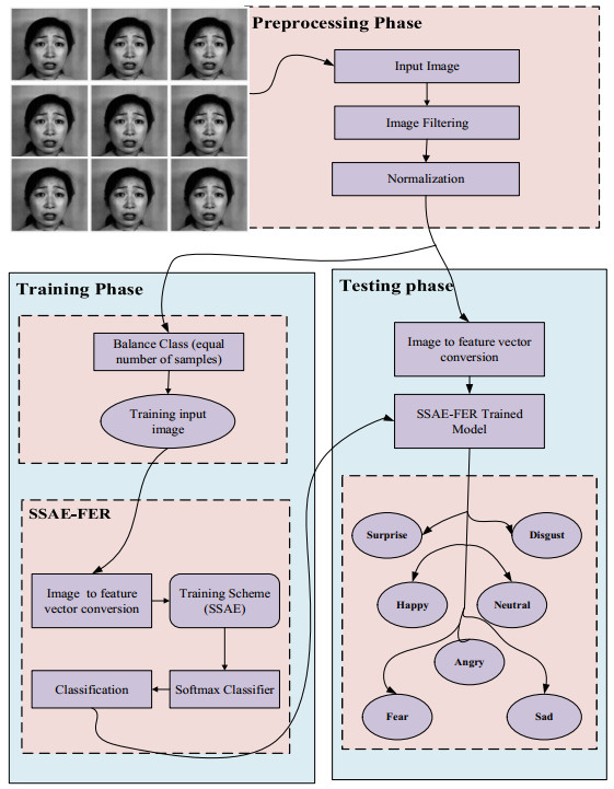
Facial expression recognition using lightweight deep learning modeling

Mubashir Ahmad; Saira; Omar Alfandi; Asad Masood Khattak; Syed Furqan Qadri; Iftikhar Ahmed Saeed; Salabat Khan; Bashir Hayat; Arshad Ahmad; Mubashir Ahmad; Saira; Omar Alfandi; Asad Masood Khattak; Syed Furqan Qadri; Iftikhar Ahmed Saeed; Salabat Khan; Bashir Hayat; Arshad Ahmad

doi:10.3934/mbe.2023357

Mathematical Biosciences and Engineering

2023, Volume 20, Issue 5: 8208-8225. doi: 10.3934/mbe.2023357

Previous Article Next Article

Research article Special Issues

Facial expression recognition using lightweight deep learning modeling

1.
Department of Computer Science, COMSATS University Islamabad, Abbottabad Campus, Tobe Camp, Abbottabad-22060, Pakistan
2.
Department of Computer Science, the University of Lahore, Sargodha Campus 40100, Pakistan
3.
College of Technological Innovation at Zayed University in Abu Dhabi, UAE
4.
Research Center for Healthcare Data Science, Zhejiang Lab, Hangzhou 311121, China
5.
College of Computer Science & Software Engineering, Shenzhen University, Shenzhen 518060, China
6.
Department of Computer Science, Institute of Management Sciences, Peshawar, Pakistan
7.
Department of IT & CS, Pak-Austria Fachhochschule: Institute of Applied Sciences and Technology (PAF-IAST), Haripur 22620, Pakistan

Academic Editor: Víctor Leiva
† These two authors contributed equally.
Correction of: Mathematical Biosciences and Engineering 20: 10675-10677

Received: 30 December 2022 Revised: 05 February 2023 Accepted: 09 February 2023 Published: 27 February 2023

Facial expression is a type of communication and is useful in many areas of computer vision, including intelligent visual surveillance, human-robot interaction and human behavior analysis. A deep learning approach is presented to classify happy, sad, angry, fearful, contemptuous, surprised and disgusted expressions. Accurate detection and classification of human facial expression is a critical task in image processing due to the inconsistencies amid the complexity, including change in illumination, occlusion, noise and the over-fitting problem. A stacked sparse auto-encoder for facial expression recognition (SSAE-FER) is used for unsupervised pre-training and supervised fine-tuning. SSAE-FER automatically extracts features from input images, and the softmax classifier is used to classify the expressions. Our method achieved an accuracy of 92.50% on the JAFFE dataset and 99.30% on the CK+ dataset. SSAE-FER performs well compared to the other comparative methods in the same domain.
- classification,
- deep learning,
- facial expression recognition,
- machine learning,
- stacked sparse auto-encoder
Citation: Mubashir Ahmad, Saira, Omar Alfandi, Asad Masood Khattak, Syed Furqan Qadri, Iftikhar Ahmed Saeed, Salabat Khan, Bashir Hayat, Arshad Ahmad. Facial expression recognition using lightweight deep learning modeling[J]. Mathematical Biosciences and Engineering, 2023, 20(5): 8208-8225. doi: 10.3934/mbe.2023357

Related Papers:

Abstract

Facial expression is a type of communication and is useful in many areas of computer vision, including intelligent visual surveillance, human-robot interaction and human behavior analysis. A deep learning approach is presented to classify happy, sad, angry, fearful, contemptuous, surprised and disgusted expressions. Accurate detection and classification of human facial expression is a critical task in image processing due to the inconsistencies amid the complexity, including change in illumination, occlusion, noise and the over-fitting problem. A stacked sparse auto-encoder for facial expression recognition (SSAE-FER) is used for unsupervised pre-training and supervised fine-tuning. SSAE-FER automatically extracts features from input images, and the softmax classifier is used to classify the expressions. Our method achieved an accuracy of 92.50% on the JAFFE dataset and 99.30% on the CK+ dataset. SSAE-FER performs well compared to the other comparative methods in the same domain.

References

[1]	A. T. Lopes, E. D. Aguiar, A. F. D. Souza, T. Oliveira-Santos, Facial expression recognition with convolutional neural networks: coping with few data and the training sample order, Pattern Recognit., 61 (2017), 610–628. https://doi.org/10.1016/j.patcog.2016.07.026 doi: 10.1016/j.patcog.2016.07.026
[2]	S. S. Hammed, A. Sabanayagam, E. Ramakalaivani, A review on facial expression recognition systems, J. Crit. Rev., 7 (2020), 903–905. Available from: https://www.jcreview.com/admin/Uploads/Files/61aa04ff88cda6.89247605.pdf.
[3]	S. Rajan, P. Chenniappan, S. Devaraj, N. Madian, Facial expression recognition techniques: a comprehensive survey, IET Image Proc., 13 (2019), 1031–1040. https://doi.org/10.1049/iet-ipr.2018.6647 doi: 10.1049/iet-ipr.2018.6647
[4]	S. H. Ma, S. M. Lai, Y. Sun, Z. C. Pan, Research status and prospect of face expression recognition, in 2019 Chinese Control And Decision Conference (CCDC), (2019), 640–646. https://doi.org/10.1109/CCDC.2019.8833483
[5]	T. A. Rashid, Convolutional neural networks based method for improving facial expression recognition, in Intelligent Systems Technologies and Applications 2016, (2016), 73–84. https://doi.org/10.1007/978-3-319-47952-1_6
[6]	M. A. Jaffar, Facial expression recognition using hybrid texture features based ensemble classifier, Int. J. Adv. Comput. Sci. Appl., 8 (2017), 449–453. https://doi.org/10.14569/IJACSA.2017.080660 doi: 10.14569/IJACSA.2017.080660
[7]	R. Gupta, Positive emotions have a unique capacity to capture attention, Prog. Brain Res., 247 (2019), 23–46. https://doi.org/10.1016/bs.pbr.2019.02.001 doi: 10.1016/bs.pbr.2019.02.001
[8]	A. B. S. Salamh, H. I. Akyüz, A new deep learning model for face recognition and registration in distance learning, Int. J. Emerging Technol. Learn., 17 (2022), 29. https://doi.org/10.3991/ijet.v17i12.30377 doi: 10.3991/ijet.v17i12.30377
[9]	M. Ahmad, D. Ai, G. Xie, S. F. Qadri, H. Song, Y. Huang, et al., Deep belief network modeling for automatic liver segmentation, IEEE Access, 7 (2019), 20585–20595. https://doi.org/10.1109/ACCESS.2019.2896961 doi: 10.1109/ACCESS.2019.2896961
[10]	S. F. Qadri, D. Ai, G. Hu, M. Ahmad, Y. Huang, Y. Wang, et al., Automatic deep feature learning via patch-based deep belief network for vertebrae segmentation in CT images, Appl. Sci., 9 (2018), 69. https://doi.org/10.3390/app9010069 doi: 10.3390/app9010069
[11]	I. Hirra, M. Ahmad, A. Hussain, M. U. Ashraf, I. A. Saeed, S. F. Qadri, et al., Breast cancer classification from histopathological images using patch-based deep learning modeling, IEEE Access, 9 (2021), 24273–24287. https://doi.org/10.1109/ACCESS.2021.3056516 doi: 10.1109/ACCESS.2021.3056516
[12]	M. Ahmad, J. Yang, D. Ai, S. F. Qadri, Y. Wang, Deep-stacked auto encoder for liver segmentation, in Advances in Image and Graphics Technologies, (2017), 243–251. https://doi.org/10.1007/978-981-10-7389-2_24
[13]	S. F. Qadri, L. Shen, M. Ahmad, S. Qadri, S. S. Zareen, M. A. Akbar, SVseg: stacked sparse autoencoder-based patch classification modeling for vertebrae segmentation, Mathematics, 10 (2022), 796. https://doi.org/10.3390/math10050796 doi: 10.3390/math10050796
[14]	M. Ahmad, S. F. Qadri, S. Qadri, I. A. Saeed, S. S. Zareen, Z. Iqbal, et al., A lightweight convolutional neural network model for liver segmentation in medical diagnosis, Comput. Intell. Neurosci., 2022 (2022), 7954333. https://doi.org/10.1155/2022/7954333 doi: 10.1155/2022/7954333
[15]	M. Ahmad, S. F. Qadri, M. U. Ashraf, K. Subhi, S. Khan, S. S. Zareen, et al., Efficient liver segmentation from computed tomography images using deep learning, Comput. Intell. Neurosci., 2022 (2022), 2665283. https://doi.org/10.1155/2022/2665283 doi: 10.1155/2022/2665283
[16]	S. F. Qadri, M. Ahmad, D. Ai, J. Yang, Y. Wang, Deep belief network based vertebra segmentation for CT images, in Image and Graphics Technologies and Applications, (2018), 536–545. https://doi.org/10.1007/978-981-13-1702-6_53
[17]	M. Ahmad, Y. Ding, S. F. Qadri, J. Yang, Convolutional-neural-network-based feature extraction for liver segmentation from CT images, in Eleventh International Conference on Digital Image Processing (ICDIP 2019), 11179 (2019), 829–835. https://doi.org/10.1117/12.2540175
[18]	I. Banerjee, Y. Ling, M. C. Chen, S. A. Hasan, C. P. Langlotz, M. Moradzadeh, et al., Comparative effectiveness of convolutional neural network (CNN) and recurrent neural network (RNN) architectures for radiology text report classification, Artif. Intell. Med., 97 (2019), 79–88. https://doi.org/10.1016/j.artmed.2018.11.004 doi: 10.1016/j.artmed.2018.11.004
[19]	M. Murugappan, A. M. Mutawa, S. Sruthi, A. Hassouneh, A. Abdulsalam, S. Jerritta, et al., Facial expression classification using KNN and decision tree classifiers, in 2020 4th International Conference on Computer, Communication and Signal Processing (ICCCSP), (2020), 1–6. https://doi.org/10.1109/ICCCSP49186.2020.9315234
[20]	M. Qasim, M. Khan, W. Mehmood, F. Sobieczky, M. Pichler, B. Moser, A comparative analysis of anomaly detection methods for predictive maintenance in SME, in Database and Expert Systems Applications - DEXA 2022 Workshops, (2022), 22–31. https://doi.org/10.1007/978-3-031-14343-4_3
[21]	M. Khan, A. Ahmad, F. Sobieczky, M. Pichler, B. A. Moser, I. Bukovský, A systematic mapping study of predictive maintenance in SMEs, IEEE Access, 10 (2022), 88738–88749. https://doi.org/10.1109/ACCESS.2022.3200694 doi: 10.1109/ACCESS.2022.3200694
[22]	W. Rafique, M. Khan, N. Sarwar, M. Sohail, A. Irshad, A graph theory based method to extract social structure in the society, in Intelligent Technologies and Applications, (2018), 437–448. https://doi.org/10.1007/978-981-13-6052-7_38
[23]	M. Khan, M. Liu, W. Dou, S. Yu, vGraph: graph virtualization towards big data, in 2015 Third International Conference on Advanced Cloud and Big Data, (2015) 153–158. https://doi.org/10.1109/CBD.2015.33
[24]	W. Rafique, M. Khan, X. Zhao, N. Sarwar, W. Dou, A blockchain-based framework for information security in intelligent transportation systems, in Intelligent Technologies and Applications, (2019), 53–66. https://doi.org/10.1007/978-981-15-5232-8_6
[25]	P. Haindl, G. Buchgeher, M. Khan, B. Moser, Towards a reference software architecture for human-AI teaming in smart manufacturing, in Proceedings of the ACM/IEEE 44th International Conference on Software Engineering: New Ideas and Emerging Results, (2022), 96–100. https://doi.org/10.1145/3510455.3512788
[26]	W. Rafique, M. Khan, W. Dou, Maintainable software solution development using collaboration between architecture and requirements in heterogeneous IoT paradigm (Short Paper), in Collaborative Computing: Networking, Applications and Worksharing, (2019), 489–508. https://doi.org/10.1007/978-3-030-30146-0_34
[27]	W. Rafique, M. Khan, N. Sarwar, W. Dou, SocioRank: A community and role detection method in social networks, Comput. Electr. Eng.*, 76 (2019), 122–132. https://doi.org/10.1016/j.compeleceng.2019.03.010 doi: 10.1016/j.compeleceng.2019.03.010
[28]	Z. Hu, J. Tang, P. Zhang, J. Jiang, Deep learning for the identification of bruised apples by fusing 3D deep features for apple grading systems, Mech. Syst. Signal Process., 145 (2020), 106922. https://doi.org/10.1016/j.ymssp.2020.106922 doi: 10.1016/j.ymssp.2020.106922
[29]	M. Iqtait, F. Mohamad, M. Mamat, Feature extraction for face recognition via active shape model (ASM) and active appearance model (AAM), IOP Conf. Ser.: Mater. Sci. Eng., 332 (2018), 012032. https://doi.org/10.1088/1757-899X/332/1/012032 doi: 10.1088/1757-899X/332/1/012032
[30]	H. Jung, S. Lee, J. Yim, S. Park, J. Kim, Joint fine-tuning in deep neural networks for facial expression recognition, in 2015 IEEE International Conference on Computer Vision (ICCV), (2015), 2983–2991. https://doi.org/10.1109/ICCV.2015.341
[31]	M. J. Cossetin, J. C. Nievola, A. L. Koerich, Facial expression recognition using a pairwise feature selection and classification approach, in 2016 International Joint Conference on Neural Networks (IJCNN), (2016), 5149–5155. https://doi.org/10.1109/IJCNN.2016.7727879
[32]	X. Zhao, X. Liang, L. Liu, T. Li, Y. Han, N. Vasconcelos, et al., Peak-piloted deep network for facial expression recognition, in Computer Vision – ECCV 2016, (2016), 425–442. https://doi.org/10.1007/978-3-319-46475-6_27
[33]	R. N. Abiram, P. Vincent, Identity preserving multi-pose facial expression recognition using fine tuned VGG on the latent space vector of generative adversarial network, Math. Biosci. Eng., 18 (2021), 3699–3717. https://doi.org/10.3934/mbe.2021186 doi: 10.3934/mbe.2021186
[34]	H. Yang, L. Yin, CNN based 3D facial expression recognition using masking and landmark features, in 2017 Seventh International Conference on Affective Computing and Intelligent Interaction (ACII), (2017), 556–560. https://doi.org/10.1109/ACII.2017.8273654
[35]	W. Wei, Q. Jia, G. Chen, Real-time facial expression recognition for affective computing based on Kinect, in 2016 IEEE 11th Conference on Industrial Electronics and Applications (ICIEA), (2016), 161–165. https://doi.org/10.1109/ICIEA.2016.7603570
[36]	B. Huang, Z. Ying, Sparse autoencoder for facial expression recognition, in 2015 IEEE 12th Intl Conf on Ubiquitous Intelligence and Computing and 2015 IEEE 12th Intl Conf on Autonomic and Trusted Computing and 2015 IEEE 15th Intl Conf on Scalable Computing and Communications and Its Associated Workshops (UIC-ATC-ScalCom), (2015), 1529–1532. https://doi.org/10.1109/UIC-ATC-ScalCom-CBDCom-IoP.2015.274
[37]	T. Ahmad, H. Mao, L. Lin, G. Tang, Action recognition using attention-joints graph convolutional neural networks, IEEE Access, 8 (2019), 305–313. https://doi.org/10.1109/ACCESS.2019.2961770 doi: 10.1109/ACCESS.2019.2961770
[38]	M. Wang, T. C. Yeh, Human action recognition using CNN and BoW methods, 2016. Available from: http://cs229.stanford.edu/proj2016spr/report/053.pdf.
[39]	C. Shen, K. Zhang, J. Tang, A covid-19 detection algorithm using deep features and discrete social learning particle swarm optimization for edge computing devices, ACM Trans. Internet Technol., 22 (2021), 1–17. https://doi.org/10.1145/3453170 doi: 10.1145/3453170
[40]	R. K. Meleppat, C. R. Fortenbach, Y. Jian, E. S. Martinez, K. Wagner, B. S. Modjtahedi, et al., In Vivo imaging of retinal and choroidal morphology and vascular plexuses of vertebrates using swept-source optical coherence tomography, Transl. Vision Sci. Technol., 11 (2022), 11. https://doi.org/10.1167/tvst.11.8.11 doi: 10.1167/tvst.11.8.11
[41]	K. Ratheesh, L. Seah, V. Murukeshan, Spectral phase-based automatic calibration scheme for swept source-based optical coherence tomography systems, Phys. Med. Biol., 61 (2016), 7652. https://doi.org/10.1088/0031-9155/61/21/7652 doi: 10.1088/0031-9155/61/21/7652
[42]	R. Meleppat, M. Matham, L. Seah, An efficient phase analysis-based wavenumber linearization scheme for swept source optical coherence tomography systems, Laser Phys. Lett., 12 (2015), 055601. https://doi.org/10.1088/1612-2011/12/5/055601 doi: 10.1088/1612-2011/12/5/055601
[43]	R. K. Meleppat, P. Prabhathan, S. L. Keey, M. V. Matham, Plasmon resonant silica-coated silver nanoplates as contrast agents for optical coherence tomography, J. Biomed. Nanotechnol., 12 (2016), 1929–1937. https://doi.org/10.1166/jbn.2016.2297 doi: 10.1166/jbn.2016.2297
[44]	D. Girish, V. Singh, A. Ralescu, Understanding action recognition in still images, in 2020 IEEE/CVF Conference on Computer Vision and Pattern Recognition Workshops (CVPRW), (2020), 1523–1529. https://doi.org/10.1109/CVPRW50498.2020.00193
[45]	H. Yang, U. Ciftci, L. Yin, Facial expression recognition by de-expression residue learning, in 2018 IEEE/CVF Conference on Computer Vision and Pattern Recognition, (2018), 2168–2177. https://doi.org/10.1109/CVPR.2018.00231
[46]	Y. Zhou, B. E. Shi, Photorealistic facial expression synthesis by the conditional difference adversarial autoencoder, in 2017 Seventh International Conference on Affective Computing and Intelligent Interaction (ACII), (2017), 370–376. https://doi.org/10.1109/ACII.2017.8273626
[47]	B. Yan, G. Han, Effective feature extraction via stacked sparse autoencoder to improve intrusion detection system, IEEE Access, 6 (2018), 41238–41248. https://doi.org/10.1109/ACCESS.2018.2858277 doi: 10.1109/ACCESS.2018.2858277
[48]	S. R. Livingstone, F. A. Russo, The Ryerson Audio-Visual Database of Emotional Speech and Song (RAVDESS): a dynamic, multimodal set of facial and vocal expressions in North American English, PloS One, 13 (2018), e0196391. https://doi.org/10.1371/journal.pone.0196391 doi: 10.1371/journal.pone.0196391
[49]	M. F. H. Siddiqui, A. Y. Javaid, A multimodal facial emotion recognition framework through the fusion of speech with visible and infrared images, Multimodal Technol. Interact., 4 (2020), 46. https://doi.org/10.3390/mti4030046 doi: 10.3390/mti4030046
[50]	J. Jang, D. H. Kim, H. I. Kim, Y. M. Ro, Color channel-wise recurrent learning for facial expression recognition, in 2017 IEEE International Conference on Acoustics, Speech and Signal Processing (ICASSP), (2017), 1233–1237. https://doi.org/10.1109/ICASSP.2017.7952353
[51]	S. Happy, A. Routray, Robust facial expression classification using shape and appearance features, in 2015 Eighth International Conference on Advances in Pattern Recognition (ICAPR), (2015), 1–5. https://doi.org/10.1109/ICAPR.2015.7050661
[52]	K. M. Koo, E. Y. Cha, Image recognition performance enhancements using image normalization, Hum.-centric Comput. Inf. Sci., 7 (2017), 33. https://doi.org/10.1186/s13673-017-0114-5 doi: 10.1186/s13673-017-0114-5
[53]	Y. Liu, Y. Li, X. Ma, R. Song, Facial expression recognition with fusion features extracted from salient facial areas, Sensors, 17 (2017), 712. https://doi.org/10.3390/s17040712 doi: 10.3390/s17040712
[54]	A. Ng, J. Ngiam, C. Y. Foo, Y. Mai, C. Suen, A. Coates, et al., Unsupervised feature learning and deep learning, 2013. Available from: https://redirect.cs.umbc.edu/courses/pub/www/courses/graduate/678/spring15/visionaudio.pdf.
[55]	L. Chen, M. Zhou, W. Su, M. Wu, J. She, K. Hirota, Softmax regression based deep sparse autoencoder network for facial emotion recognition in human-robot interaction, Inf. Sci., 428 (2018), 49–61. https://doi.org/10.1016/j.ins.2017.10.044 doi: 10.1016/j.ins.2017.10.044
[56]	M. J. Lyons, “Excavating AI” Re-excavated: Debunking a fallacious account of the JAFFE dataset, preprint, arXiv:2107.13998.
[57]	M. J. Lyons, M. Kamachi, J. Gyoba, Coding facial expressions with Gabor wavelets (IVC special issue), preprint, arXiv:2009.05938.
[58]	T. Kanade, J. F. Cohn, Y. Tian, Comprehensive database for facial expression analysis, in Proceedings Fourth IEEE International Conference on Automatic Face and Gesture Recognition (Cat. No. PR00580), (2000), 46–53. https://doi.org/10.1109/AFGR.2000.840611
[59]	S. Eng, H. Ali, A. Cheah, Y. Chong, Facial expression recognition in JAFFE and KDEF datasets using histogram of oriented gradients and support vector machine, in IOP Conf. Ser.: Mater. Sci. Eng., 705 (2019), 012031. https://doi.org/10.1088/1757-899X/705/1/012031
[60]	R. B. Palm, Prediction as a candidate for learning deep hierarchical models of data, 2012. Available from: https://www2.imm.dtu.dk/pubdb/edoc/imm6284.pdf.
[61]	L. Du, H. Hu, Modified classification and regression tree for facial expression recognition with using difference expression images, Electron. Lett., 53 (2017), 590–592. https://doi.org/10.1049/el.2017.0731 doi: 10.1049/el.2017.0731
[62]	V. H. Duong, Y. S. Lee, J. J. Ding, B. T. Pham, M. Q. Bui, J. C. Wang, Projective complex matrix factorization for facial expression recognition, EURASIP J. Adv. Signal Process., 2018 (2018), 10. https://doi.org/10.1186/s13634-017-0521-9 doi: 10.1186/s13634-017-0521-9
[63]	T. Zhang, Face expression recognition based on deep learning, J. Phys.: Conf. Ser., 1486 (2020), 042048. https://doi.org/10.1088/1742-6596/1486/4/042048 doi: 10.1088/1742-6596/1486/4/042048

Reader Comments

Your name:*

Email:*
© 2023 the Author(s), licensee AIMS Press. This is an open access article distributed under the terms of the Creative Commons Attribution License (http://creativecommons.org/licenses/by/4.0)