A topical VAEGAN-IHMM approach for automatic story segmentation

Jia Yu; Huiling Peng; Guoqiang Wang; Nianfeng Shi; Jia Yu; Huiling Peng; Guoqiang Wang; Nianfeng Shi

doi:10.3934/mbe.2024289

Mathematical Biosciences and Engineering

2024, Volume 21, Issue 7: 6608-6630. doi: 10.3934/mbe.2024289

Previous Article Next Article

Research article Special Issues

A topical VAEGAN-IHMM approach for automatic story segmentation

1.
School of Computer and Information Engineering, Luoyang Institute of Science and Technology, China
2.
Software Research Institute, Technological University of Shannon, Ireland

Received: 15 February 2024 Revised: 18 June 2024 Accepted: 27 June 2024 Published: 16 July 2024

Feature representations with rich topic information can greatly improve the performance of story segmentation tasks. VAEGAN offers distinct advantages in feature learning by combining variational autoencoder (VAE) and generative adversarial network (GAN), which not only captures intricate data representations through VAE's probabilistic encoding and decoding mechanism but also enhances feature diversity and quality via GAN's adversarial training. To better learn topical domain representation, we used a topical classifier to supervise the training process of VAEGAN. Based on the learned feature, a segmentor splits the document into shorter ones with different topics. Hidden Markov model (HMM) is a popular approach for story segmentation, in which stories are viewed as instances of topics (hidden states). The number of states has to be set manually but it is often unknown in real scenarios. To solve this problem, we proposed an infinite HMM (IHMM) approach which utilized an HDP prior on transition matrices over countably infinite state spaces to automatically infer the state's number from the data. Given a running text, a Blocked Gibbis sampler labeled the states with topic classes. The position where the topic changes was a story boundary. Experimental results on the TDT2 corpus demonstrated that the proposed topical VAEGAN-IHMM approach was significantly better than the traditional HMM method in story segmentation tasks and achieved state-of-the-art performance.
- generative adversarial network,
- variational autoencoder,
- HDP,
- hidden Markov model,
- story segmentation
Citation: Jia Yu, Huiling Peng, Guoqiang Wang, Nianfeng Shi. A topical VAEGAN-IHMM approach for automatic story segmentation[J]. Mathematical Biosciences and Engineering, 2024, 21(7): 6608-6630. doi: 10.3934/mbe.2024289

Related Papers:

Abstract

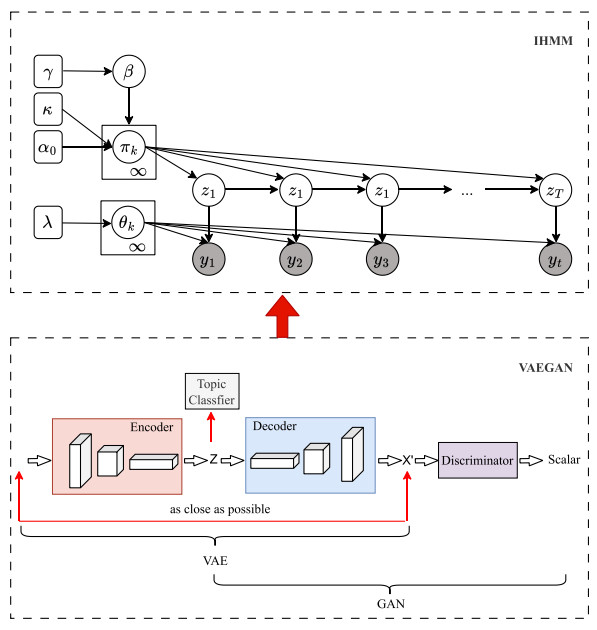
Feature representations with rich topic information can greatly improve the performance of story segmentation tasks. VAEGAN offers distinct advantages in feature learning by combining variational autoencoder (VAE) and generative adversarial network (GAN), which not only captures intricate data representations through VAE's probabilistic encoding and decoding mechanism but also enhances feature diversity and quality via GAN's adversarial training. To better learn topical domain representation, we used a topical classifier to supervise the training process of VAEGAN. Based on the learned feature, a segmentor splits the document into shorter ones with different topics. Hidden Markov model (HMM) is a popular approach for story segmentation, in which stories are viewed as instances of topics (hidden states). The number of states has to be set manually but it is often unknown in real scenarios. To solve this problem, we proposed an infinite HMM (IHMM) approach which utilized an HDP prior on transition matrices over countably infinite state spaces to automatically infer the state's number from the data. Given a running text, a Blocked Gibbis sampler labeled the states with topic classes. The position where the topic changes was a story boundary. Experimental results on the TDT2 corpus demonstrated that the proposed topical VAEGAN-IHMM approach was significantly better than the traditional HMM method in story segmentation tasks and achieved state-of-the-art performance.

References

[1]	U. R. Gondhi, Intra-Topic Clustering for Social Media, 2020.
[2]	M. Adedoyin-Olowe, M. M. Gaber, F. Stahl, A survey of data mining techniques for social media analysis, J. Data Mining Digital Humanit., 2014 (2014). https://doi.org/10.46298/jdmdh.5 doi: 10.46298/jdmdh.5
[3]	L. F. Rau, P. S. Jacobs, U. Zernik, Information extraction and text summarization using linguistic knowledge acquisition, Inf. Process. Manage., 25 (1989), 419–428. https://doi.org/10.1016/0306-4573(89)90069-1 doi: 10.1016/0306-4573(89)90069-1
[4]	L. Lee, B. Chen, Spoken document understanding and organization, IEEE Signal Process. Mag., 22 (2005), 42–60.
[5]	W. Dan, C. Liu, Eye tracking analysis in interactive information retrieval research, J. Libr. Sci. China, 2 (2019), 109–128.
[6]	B. Zhang, Z. Chen, D. Peng, J. A. Benediktsson, B. Liu, L. Zhou, et al., Remotely sensed big data: Evolution in model development for information extraction[point of view], Proc. IEEE, 107 (2019), 2294–2301. https://doi.org/10.1109/JPROC.2019.2948454 doi: 10.1109/JPROC.2019.2948454
[7]	S. Soderland, Learning information extraction rules for semi-structured and free text, Mach. Learn., 34 (1999), 233–272. https://doi.org/10.1023/A:1007562322031 doi: 10.1023/A:1007562322031
[8]	W. Chen, B. Liu, W. Guan, ERNIE and multi-feature fusion for news topic classification, Artif. Intell. Appl., 2 (2024), 149–154. https://doi.org/10.47852/bonviewAIA32021743 doi: 10.47852/bonviewAIA32021743
[9]	W. Hsu, L. Kennedy, C. W. Huang, S. F. Chang, C. Y. Lin, G. Iyengar, News video story segmentation using fusion of multi-level multi-modal features in trecvid 2003, in 2004 IEEE International Conference on Acoustics, Speech, and Signal Processing, IEEE, (2004), 645.
[10]	J. Wan, T. Peng, B. Li, News video story segmentation based on naive bayes model, in 2009 Fifth International Conference on Natural Computation, IEEE, (2009), 77–81.
[11]	G. Hadjeres, F. Nielsen, F. Pachet, GLSR-VAE: Geodesic latent space regularization for variational autoencoder architectures, in 2017 IEEE Symposium Series on Computational Intelligence (SSCI), IEEE, (2017), 1–7. https://doi.org/10.1109/SSCI.2017.8280895
[12]	I. Malioutov, A. Park, R. Barzilay, J. Glass, Making sense of sound: Unsupervised topic segmentation over acoustic input, in Proceedings of the 45th Annual Meeting of the Association of Computational Linguistics, (2007), 504–511.
[13]	L. Chaisorn, T. S. Chua, C. H. Lee, A multi-modal approach to story segmentation for news video, World Wide Web, 6 (2003), 187–208. https://doi.org/10.1023/A:1023622605600 doi: 10.1023/A:1023622605600
[14]	S. Banerjee, A. Rudnicky, A TextTiling based approach to topic boundary detection in meetings, Proc. Interspeech 2006, (2006), 1827. https://doi.org/10.21437/Interspeech.2006-15 doi: 10.21437/Interspeech.2006-15
[15]	I. I. M. Malioutov, Minimum cut model for spoken lecture segmentation, in ACL-44: Proceedings of the 21st International Conference on Computational Linguistics and the 44th annual meeting of the Association for Computational Linguistics, (2006), 25–32. https://doi.org/10.3115/1220175.1220179
[16]	S. S. Naziya, R. Deshmukh, Speech recognition system—A review, IOSR J. Comput. Eng., 18 (2016), 3–8. https://doi.org/10.9790/0661-1804020109 doi: 10.9790/0661-1804020109
[17]	L. Li, Y. Zhao, D. Jiang, Y. Zhang, F. Wang, I. Gonzalez, et al., Hybrid deep neural network--hidden markov model (DNN-HMM) based speech emotion recognition, in 2013 Humaine Association Conference on Affective Computing and Intelligent Interaction, IEEE, (2013), 312–317.
[18]	Z. S. Harris, Distributional structure, Word, 10 (1954), 146–162. https://doi.org/10.1080/00437956.1954.11659520 doi: 10.1080/00437956.1954.11659520
[19]	Y. Zhang, R. Jin, Z. H. Zhou, Understanding bag-of-words model: A statistical framework, Int. J. Mach. Learn. Cybern., 1 (2010), 43–52. https://doi.org/10.1007/s13042-010-0001-0 doi: 10.1007/s13042-010-0001-0
[20]	A. Alahmadi, A. Joorabchi, A. E. Mahdi, A new text representation scheme combining bag-of-words and bag-of-concepts approaches for automatic text classification, in 2013 7th IEEE GCC Conference and Exhibition (GCC), IEEE, (2013), 108–113. https://doi.org/10.1109/IEEEGCC.2013.6705759
[21]	Q. Le, T. Mikolov, Distributed representations of sentences and documents, in International Conference on Machine Learning, PMLR, (2014), 1188–1196.
[22]	Y. M. Costa, L. S. Oliveira, C. N. Silla Jr, An evaluation of convolutional neural networks for music classification using spectrograms, Appl. Soft Comput., 52 (2017), 28–38. https://doi.org/10.1016/j.asoc.2016.12.024 doi: 10.1016/j.asoc.2016.12.024
[23]	J. Yu, X. Xiao, L. Xie, E. S. Chng, H. Li, A DNN-HMM approach to story segmentation, Proc. Interspeech, (2016), 1527–1531.
[24]	L. Xie, Y. L. Yang, Z. Q. Liu, On the effectiveness of subwords for lexical cohesion based story segmentation of Chinese broadcast news, Inf. Sci., 181 (2011), 2873–2891. https://doi.org/10.1016/j.ins.2011.02.013 doi: 10.1016/j.ins.2011.02.013
[25]	L. Xie, Y. Yang, J. Zeng, Subword lexical chaining for automatic story segmentation in Chinese broadcast news, in Lecture Notes in Computer Science, Springer, (2008), 248–258. https://doi.org/10.1007/978-3-540-89796-5_26
[26]	H. Yu, J. Yang, A direct LDA algorithm for high-dimensional data—with application to face recognition, Pattern Recognit., 34 (2001), 2067–2070. https://doi.org/10.1016/S0031-3203(00)00162-X doi: 10.1016/S0031-3203(00)00162-X
[27]	M. Lu, L. Zheng, C. C. Leung, L. Xie, B. Ma, H. Li, Broadcast news story segmentation using probabilistic latent semantic analysis and laplacian eigenmaps, in APSIPA ASC 2011, (2011), 356–360.
[28]	T. Hofmann, Probabilistic latent semantic indexing, in Proceedings of the 22nd Annual International ACM SIGIR Conference on Research and Development in Information Retrieval, (1999), 50–57. https://doi.org/10.1145/312624.312649
[29]	L. Manevitz, M. Yousef, One-class document classification via neural networks, Neurocomputing, 70 (2007), 1466–1481. https://doi.org/10.1016/j.neucom.2006.05.013 doi: 10.1016/j.neucom.2006.05.013
[30]	Y. Cheng, Z. Ye, M. Wang, Q. Zhang, Document classification based on convolutional neural network and hierarchical attention network, Neural Network World, 29 (2019). https://doi.org/10.14311/NNW.2019.29.007 doi: 10.14311/NNW.2019.29.007
[31]	C. H. Li, S. C. Park, An efficient document classification model using an improved back propagation neural network and singular value decomposition, Expert Syst. Appl., 36 (2009), 3208–3215. https://doi.org/10.1016/j.eswa.2008.01.014 doi: 10.1016/j.eswa.2008.01.014
[32]	Q. Yao, Q. Liu, T. G. Dietterich, S. Todorovic, J. Lin, G. Diao, et al., Segmentation of touching insects based on optical flow and NCuts, Biosyst. Eng., 114 (2013), 67–77. https://doi.org/10.1016/j.biosystemseng.2012.11.008 doi: 10.1016/j.biosystemseng.2012.11.008
[33]	Y. Cen, Z. Han, P. Ji, Chinese term recognition based on hidden Markov model, in 2008 IEEE Pacific-Asia Workshop on Computational Intelligence and Industrial Application, (2008), 54–58. https://doi.org/10.1109/PACⅡA.2008.242
[34]	J. P. Yamron, I. Carp, L. Gillick, S. Lowe, P. van Mulbregt, A hidden Markov model approach to text segmentation and event tracking, in Proceedings of the 1998 IEEE International Conference on Acoustics, Speech and Signal Processing, (1998), 333–336.
[35]	F. Lan, Research on text similarity measurement hybrid algorithm with term semantic information and TF‐IDF Method, Adv. Multimedia, (2022), 7923262. https://doi.org/10.1155/2022/7923262 doi: 10.1155/2022/7923262
[36]	J. Yu, H. Shao, Broadcast news story segmentation using sticky hierarchical dirichlet process, Appl. Intell., 2 (2022), 12788–12800. https://doi.org/10.1007/s10489-021-03098-4 doi: 10.1007/s10489-021-03098-4
[37]	C. E. Antoniak, Mixtures of Dirichlet processes with applications to Bayesian nonparametric problems, Ann. Stat., (1974), 1152–1174. https://doi.org/10.1214/aos/1176342871 doi: 10.1214/aos/1176342871
[38]	D. M. Blei, M. I. Jordan, Variational Inference for Dirichlet Process Mixtures, (2006).
[39]	M. D. Hoffman, P. R. Cook, D. M. Blei, Data-driven recomposition using the hierarchical Dirichlet process hidden Markov model, ICMC, (2008).
[40]	Y. W. Teh, Dirichlet process, encyclopedia of machine learning, 1063 (2010), 280–287. https://doi.org/10.1007/978-0-387-30164-8_219
[41]	W. M. Bolstad, Understanding Computational Bayesian Statistics, John Wiley & Sons, 2009. https://doi.org/10.1002/9780470567371
[42]	G. Casella, E. I. George, Explaining the Gibbs sampler, Am. Stat., 46 (1992), 167–174. https://doi.org/10.1080/00031305.1992.10475878 doi: 10.1080/00031305.1992.10475878
[43]	C. M. Bishop, Pattern Recognition and Machine Learning, Springer, 2 (2006), 1122–1128.
[44]	T. Cohn, P. Blunsom, Blocked inference in Bayesian tree substitution grammars, in Proceedings of the ACL 2010 Conference Short Papers, (2010), 225–230.
[45]	J. Fiscus, G. Doddington, J. Garofolo, A. Martin, NIST's 1998 topic detection and tracking evaluation (TDT2), in Proceedings of the 1999 DARPA Broadcast News Workshop, (1999), 19–24. https://doi.org/10.21437/Eurospeech.1999-65
[46]	G. Karypis, CLUTO-a clustering toolkit, (2002). https://doi.org/10.21236/ADA439508
[47]	M. Lu, L. Zheng, C. Leung, L. Xie, B. Ma, H. Li, Broadcast news story segmentation using probabilistic latent semantic analysis and laplacian eigenmaps, in APSIPA ASC 2011, 356–360, (2011).
[48]	J. Eisenstein, Barzilay R, Bayesian unsupervised topic segmentation, in EMNLP '08: Proceedings of the Conference on Empirical Methods in Natural Language Processing, (2008), 334–343. https://doi.org/10.3115/1613715.1613760
[49]	C. Wei, S. Luo, X. Ma, H. Ren, J. Zhang, L. Pan, Locally embedding autoencoders: A semi-supervised manifold learning approach of document representation, PloS One, 11 (2016), e0146672. https://doi.org/10.1371/journal.pone.0146672 doi: 10.1371/journal.pone.0146672
[50]	C. Yang, L. Xie, X. Zhou. Unsupervised broadcast news story segmentation using distance dependent Chinese restaurant processes, in 2014 IEEE International Conference on Acoustics, Speech and Signal Processing (ICASSP), (2014), 4062–4066. https://doi.org/10.1109/ICASSP.2014.6854365
[51]	J. Yu, L. Xie, A hybrid neural network hidden Markov model approach for automatic story segmentation, J. Ambient Intell. Humanized Comput., 8 (2017), 925–936. https://doi.org/10.1007/s12652-017-0501-9 doi: 10.1007/s12652-017-0501-9

Reader Comments

Your name:*

Email:*
© 2024 the Author(s), licensee AIMS Press. This is an open access article distributed under the terms of the Creative Commons Attribution License (http://creativecommons.org/licenses/by/4.0)