Predator-prey systems with defense switching and density-suppressed dispersal strategy

Jiawei Chu; Hai-Yang Jin; Jiawei Chu; Hai-Yang Jin

doi:10.3934/mbe.2022582

Mathematical Biosciences and Engineering

2022, Volume 19, Issue 12: 12472-12499. doi: 10.3934/mbe.2022582

Previous Article Next Article

Research article Special Issues

Predator-prey systems with defense switching and density-suppressed dispersal strategy

Jiawei Chu ¹,
Hai-Yang Jin ^{2
,
,}

1.
Department of Applied Mathematics, The Hong Kong Polytechnic University, Hung Hom, Hong Kong, China
2.
School of Mathematics, South China University of Technology, Guangzhou 510640, China

Academic Editor: Yong Jung Kim

Received: 19 June 2022 Revised: 07 August 2022 Accepted: 12 August 2022 Published: 26 August 2022

In this paper, we consider the following predator-prey system with defense switching mechanism and density-suppressed dispersal strategy

$ \begin{equation*} \begin{cases} u_t = \Delta(d_1(w)u)+\frac{\beta_1 uvw}{u+v}-\alpha_1 u, & x\in \Omega, \; \; t>0, \\ v_t = \Delta(d_2(w)v)+\frac{\beta_2 uvw}{u+v}-\alpha_2 v, & x\in \Omega, \; \; t>0, \\ w_t = \Delta w-\frac{\beta_3 uvw}{u+v}+\sigma w\left(1-\frac{w}{K}\right), & x\in \Omega, \; \; t>0, \\ \frac{\partial u}{\partial \nu} = \frac{\partial v}{\partial \nu} = \frac{\partial w}{\partial \nu} = 0, & x\in\partial\Omega, \; \; t>0, \\ (u, v, w)(x, 0) = (u_0, v_0, w_0)(x), & x\in\Omega, \ \end{cases} \end{equation*} $

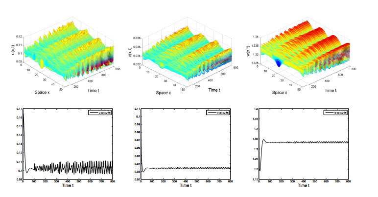
where $ \Omega\subset{\mathbb{R}}^2 $ is a bounded domain with smooth boundary. Based on the method of energy estimates and Moser iteration, we establish the existence of global classical solutions with uniform-in-time boundedness. We further prove the global stability of co-existence equilibrium by using the Lyapunov functionals and LaSalle's invariant principle. Finally we conduct linear stability analysis and perform numerical simulations to illustrate that the density-suppressed dispersal may trigger the pattern formation.
- prey-predator system,
- defense switching,
- density-suppressed diffusion,
- global stability,
- pattern formation
Citation: Jiawei Chu, Hai-Yang Jin. Predator-prey systems with defense switching and density-suppressed dispersal strategy[J]. Mathematical Biosciences and Engineering, 2022, 19(12): 12472-12499. doi: 10.3934/mbe.2022582

Related Papers:

Abstract

In this paper, we consider the following predator-prey system with defense switching mechanism and density-suppressed dispersal strategy

$ \begin{equation*} \begin{cases} u_t = \Delta(d_1(w)u)+\frac{\beta_1 uvw}{u+v}-\alpha_1 u, & x\in \Omega, \; \; t>0, \\ v_t = \Delta(d_2(w)v)+\frac{\beta_2 uvw}{u+v}-\alpha_2 v, & x\in \Omega, \; \; t>0, \\ w_t = \Delta w-\frac{\beta_3 uvw}{u+v}+\sigma w\left(1-\frac{w}{K}\right), & x\in \Omega, \; \; t>0, \\ \frac{\partial u}{\partial \nu} = \frac{\partial v}{\partial \nu} = \frac{\partial w}{\partial \nu} = 0, & x\in\partial\Omega, \; \; t>0, \\ (u, v, w)(x, 0) = (u_0, v_0, w_0)(x), & x\in\Omega, \ \end{cases} \end{equation*} $

where $ \Omega\subset{\mathbb{R}}^2 $ is a bounded domain with smooth boundary. Based on the method of energy estimates and Moser iteration, we establish the existence of global classical solutions with uniform-in-time boundedness. We further prove the global stability of co-existence equilibrium by using the Lyapunov functionals and LaSalle's invariant principle. Finally we conduct linear stability analysis and perform numerical simulations to illustrate that the density-suppressed dispersal may trigger the pattern formation.

References

[1]	M. Saleem, A. K. Tripathi, A. H. Sadiyal, Coexistence of species in a defensive switching model, Math. Biosci., 181 (2003), 145–164. https://doi.org/10.1016/S0025-5564(02)00152-9 doi: 10.1016/S0025-5564(02)00152-9
[2]	S. Takahashi, M. Hori, Unstable evolutionarily stable strategy and oscillation: A model of lateral asymmetry in scale-eating cichlids, Am. Nat., 144 (1994), 1001–1020. https://doi.org/10.1086/285722 doi: 10.1086/285722
[3]	P. Y. H. Pang, M. Wang, Strategy and stationary pattern in a three-species predator-prey model, J. Differ. Equations, 200 (2004), 245–273. https://doi.org/10.1016/j.jde.2004.01.004 doi: 10.1016/j.jde.2004.01.004
[4]	Y. Cai, Q. Cao, Z. A. Wang, Asymptotic dynamics and spatial patterns of a ratio-dependent predator-prey system with prey-taxis, Appl. Anal., 101 (2022), 81–99. https://doi.org/10.1080/00036811.2020.1728259 doi: 10.1080/00036811.2020.1728259
[5]	J. Wang, X. Guo, Dynamics and pattern formations in a three-species predator-prey model with two prey-taxis, J. Math. Anal. Appl., 475 (2019), 1054–1072. https://doi.org/10.1016/j.jmaa.2019.02.071 doi: 10.1016/j.jmaa.2019.02.071
[6]	X. Guo, J. Wang, Dynamics and pattern formations in diffusive predator-prey models with two prey-taxis, Math. Methods Appl. Sci., 42 (2019), 4197–4212. https://doi.org/10.1002/mma.5639 doi: 10.1002/mma.5639
[7]	P. Kareiva, G. Odell, Swarms of predators exhibit "preytaxis" if individual predators use area-restricted search, Am. Nat., 130 (2015), 233–270. https://doi.org/10.1086/284707 doi: 10.1086/284707
[8]	H. Y. Jin, Z. A. Wang, Global dynamics and spatio-temporal patterns of predator-prey systems with density-dependent motion, European J. Appl. Math., 32 (2021), 652–682. https://doi.org/10.1017/S0956792520000248 doi: 10.1017/S0956792520000248
[9]	Z. A. Wang, J. Xu, On the Lotka-Volterra competition system with dynamical resources and density-dependent diffusion, J. Math. Biol., 82 (2021), 1–37. https://doi.org/10.1007/s00285-021-01562-w doi: 10.1007/s00285-021-01562-w
[10]	E. Keller, L. Segel, Traveling bands of chemotactic bacteria: A theoretical analysis, J. Theor. Biol., 30 (1971), 377–380. https://doi.org/10.1016/0022-5193(71)90051-8 doi: 10.1016/0022-5193(71)90051-8
[11]	E. Keller, L. Segel, Model for chemotaxis, J. Theor. Biol., 30 (1971), 225–234. https://doi.org/10.1016/0022-5193(71)90050-6
[12]	X. Fu, L. H. Tang, C. Liu, J. D. Huang, T. Hwa, P. Lenz, Stripe formation in bacterial systems with density-suppressed motility, Phys. Rev. Lett., 108 (2012), 198102. https://doi.org/10.1103/physrevlett.108.198102 doi: 10.1103/physrevlett.108.198102
[13]	C. Liu, X. Fu, L. Liu, X. Ren, C. K. Chau, S. Li, et al., Sequential establishment of stripe patterns in an expanding cell population, Science, 334 (2011), 238–241. https://doi.org/10.1126/science.1209042 doi: 10.1126/science.1209042
[14]	J. Ahn, C. Yoon, Global well-posedness and stability of constant equilibria in parabolic-elliptic chemotaxis systems without gradient sensing, Nonlinearity, 32 (2019), 1327–1251. https://doi.org/10.1088/1361-6544/aaf513 doi: 10.1088/1361-6544/aaf513
[15]	M. Burger, P. Laurençot, A. Trescases, Delayed blow-up for chemotaxis models with local sensing, J. Lond. Math. Soc., 103 (2021), 1596–1617. https://doi.org/10.1112/jlms.12420 doi: 10.1112/jlms.12420
[16]	H. Y. Jin, Y. J. Kim, Z. A. Wang, Boundedness, stabilization, and pattern formation driven by density-suppressed motility, SIAM J. Appl. Math., 78 (2018), 1632–1657. https://doi.org/10.1137/17M1144647 doi: 10.1137/17M1144647
[17]	K. Fujie, J. Jiang, Global existence for a kinetic model of pattern formation with density-suppressed motilities, J. Differ. Equations, 269 (2020), 5338–5378. https://doi.org/10.1016/j.jde.2020.04.001 doi: 10.1016/j.jde.2020.04.001
[18]	J. Jiang, P. Laurençot, Y. Zhang, Global existence, uniform boundedness, and stabilization in a chemotaxis system with density-suppressed motility and nutrient consumption, Comm. Partial Differ. Equations, 47 (2022), 1024–1069. https://doi.org/10.1080/03605302.2021.2021422 doi: 10.1080/03605302.2021.2021422
[19]	J. Jiang, P. Laurençot, Global existence and uniform boundedness in a chemotaxis model with signal-dependent motility, J. Differ. Equations, 299 (2021), 513–541. https://doi.org/10.1016/j.jde.2021.07.029 doi: 10.1016/j.jde.2021.07.029
[20]	H. Y. Jin, Z. A. Wang, Critical mass on the Keller-Segel system with signal-dependent motility. Proc. Amer. Math. Soc., 148 (2020), 4855–4873. https://doi.org/10.1090/proc/15124
[21]	H. Y. Jin, S. Shi, Z. A. Wang, Boundedness and asymptotics of a reaction-diffusion system with density-dependent motility, J. Differ. Equations, 269 (2020), 6758–6793. https://doi.org/10.1016/j.jde.2020.05.018 doi: 10.1016/j.jde.2020.05.018
[22]	W. Lv, Q. Wang, An $n$-dimensional chemotaxis system with signal-dependent motility and generalized logistic source: global existence and asymptotic stabilization, Proc. Roy. Soc. Edinburgh Sect. A, 151 (2021), 821–841. https://doi.org/10.1017/prm.2020.38 doi: 10.1017/prm.2020.38
[23]	W. Lyu, Z.-A. Wang, Global classical solutions for a class of reaction-diffusion system with density-suppressed motility, Electron. Res. Arch., 30 (2022), 995–1015. https://doi.org/10.3934/era.2022052 doi: 10.3934/era.2022052
[24]	W. Lv, Global existence for a class of chemotaxis-consumption systems with signal-dependent motility and generalized logistic source, Nonlinear Anal. Real World Appl., 56 (2020), 103160. https://doi.org/10.1016/j.nonrwa.2020.103160 doi: 10.1016/j.nonrwa.2020.103160
[25]	J. Smith Roberge, D. Iron, T. Kolokolnikov, Pattern formation in bacterial colonies with density-dependent diffusion, European J. Appl. Math., 30 (2019), 196–218. https://doi.org/10.1017/S0956792518000013 doi: 10.1017/S0956792518000013
[26]	M. Wang, J. Wang, Boundedness in the higher-dimensional Keller-Segel model with signal-dependent motility and logistic growth, J. Math. Phys., 60 (2019), 011507. https://doi.org/10.1063/1.5061738 doi: 10.1063/1.5061738
[27]	C. Yoon, Y.-J. Kim, Global existence and aggregation in a Keller-Segel model with Fokker-Planck diffusion, Acta Appl. Math., 149 (2017), 101–123. https://doi.org/10.1007/s10440-016-0089-7 doi: 10.1007/s10440-016-0089-7
[28]	C. Xu, Y. Wang, Asymptotic behavior of a quasilinear Keller-Segel system with signal-suppressed motility, Calc. Var. Partial Differ. Equations, 60 (2021), 1–29. https://doi.org/10.1007/s00526-021-02053-y doi: 10.1007/s00526-021-02053-y
[29]	J. Li, Z.-A. Wang, Traveling wave solutions to the density-suppressed motility model, J. Differential Equations, 301 (2021), 1–36. https://doi.org/10.1016/j.jde.2021.07.038 doi: 10.1016/j.jde.2021.07.038
[30]	M. Ma, R. Peng, Z. Wang. Stationary and non-stationary patterns of the density-suppressed motility model. Phys. D, 402 (2020), 132259. https://doi.org/10.1016/j.physd.2019.132259
[31]	Z.-A. Wang, X. Xu, Steady states and pattern formation of the density-suppressed motility model, IMA J. Appl. Math., 86 (2021), 577–603. https://doi.org/10.1093/imamat/hxab006 doi: 10.1093/imamat/hxab006
[32]	A. Yagi, Abstract parabolic evolution equations and their applications, Springer Science and Business Media, 2009. https://doi.org/10.1007/978-3-642-04631-5
[33]	N. Alikakos, $L^p$ bounds of solutions of reaction-diffusion equations, , Commun. Partial Differ. Equations, 4 (1979), 827–868. https://doi.org/10.1080/03605307908820113 doi: 10.1080/03605307908820113
[34]	J. Murray, Mathematical Biology I: An Introduction, 3$^{rd}$ edition, Springer, Berlin, 2002. https://doi.org/10.1007/b98868
[35]	J. Wang, J. Shi, J. Wei, Dynamics and pattern formation in a diffusive predator-prey system with strong Allee effect in prey, J. Differ. Equations, 251 (2011), 1276–1304. https://doi.org/10.1016/j.jde.2011.03.004 doi: 10.1016/j.jde.2011.03.004
[36]	H. Amann, Dynamic theory of quasilinear parabolic equations. II. Reaction-diffusion systems, Differ. Integral Equations, 3 (1990), 13–75.
[37]	H. Amann, Nonhomogeneous linear and quasilinear elliptic and parabolic boundary value problems, Funct. Spaces Differ. Oper. Nonlinear Anal., 133 (1993), 9–126. https://doi.org/10.1007/978-3-663-11336-2_1 doi: 10.1007/978-3-663-11336-2_1
[38]	H. Y. Jin, Z. A. Wang, Global stability of prey-taxis systems, J. Differ. Equations, 262 (2017), 1257–1290. https://doi.org/10.1016/j.jde.2016.10.010 doi: 10.1016/j.jde.2016.10.010
[39]	R. Kowalczyk, Z. Szymańska, On the global existence of solutions to an aggregation model, J. Math. Anal. Appl., 343 (2008), 379–398. https://doi.org/10.1016/j.jmaa.2008.01.005 doi: 10.1016/j.jmaa.2008.01.005
[40]	P. Liu, J. Shi, Z.-A. Wang, Pattern formation of the attraction-repulsion Keller-Segel system, Discrete Contin. Dyn. Syst. Ser. B, 18 (2013), 2597–2625. https://doi.org/10.3934/dcdsb.2013.18.2597 doi: 10.3934/dcdsb.2013.18.2597
[41]	S. Sastry, Nonlinear System: Analysis, Stability, and Control, Springer, New York, 1999. https://doi.org/10.1007/978-1-4757-3108-8

Reader Comments

Your name:*

Email:*
© 2022 the Author(s), licensee AIMS Press. This is an open access article distributed under the terms of the Creative Commons Attribution License (http://creativecommons.org/licenses/by/4.0)