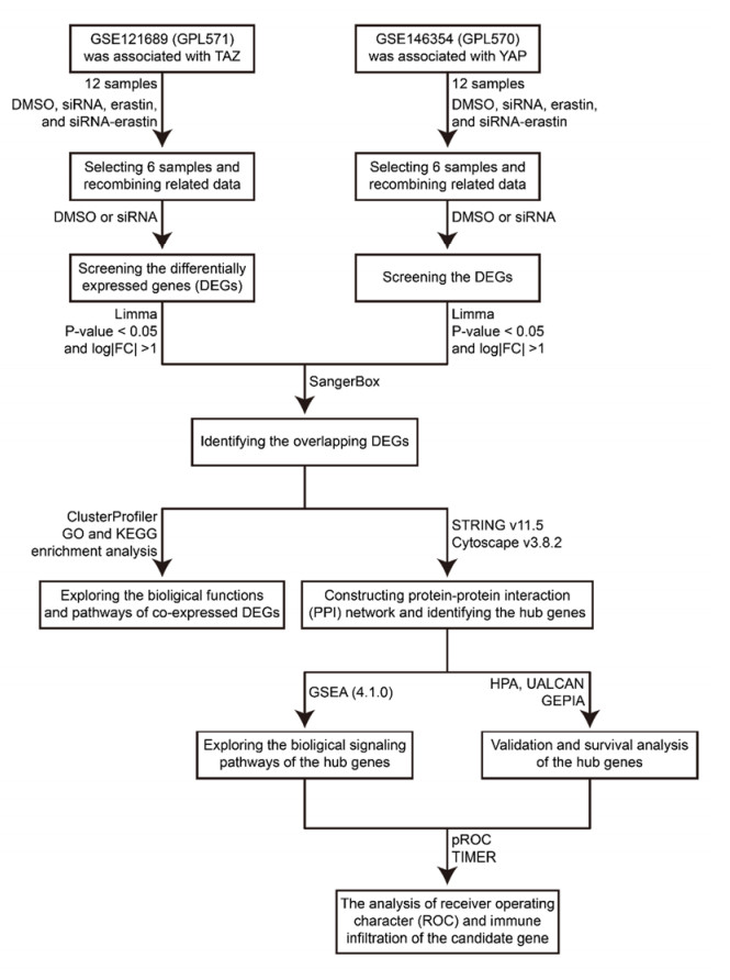
WW domain-containing transcription regulator 1 (TAZ, or WWTR1) and Yes-associated protein 1 (YAP) are both important effectors of the Hippo pathway and exhibit different functions. However, few studies have explored their co-regulatory mechanisms in kidney renal clear cell carcinoma (KIRC). Here, we used bioinformatics approaches to evaluate the co-regulatory roles of TAZ/YAP and screen novel biomarkers in KIRC. GSE121689 and GSE146354 were downloaded from the GEO. The limma was applied to identify the differential expression genes (DEGs) and the Venn diagram was utilized to screen co-expressed DEGs. Co-expressed DEGs obtained the corresponding pathways through GO and KEGG analysis. The protein-protein interaction (PPI) network was constructed using STRING. The hub genes were selected applying MCODE and CytoHubba. GSEA was further applied to identify the hub gene-related signaling pathways. The expression, survival, receiver operating character (ROC), and immune infiltration of the hub genes were analyzed by HPA, UALCAN, GEPIA, pROC, and TIMER. A total of 51 DEGs were co-expressed in the two datasets. The KEGG results showed that the enriched pathways were concentrated in the TGF-β signaling pathway and endocytosis. In the PPI network, the hub genes (STAU2, AGO2, FMR1) were identified by the MCODE and CytoHubba. The GSEA results revealed that the hub genes were correlated with the signaling pathways of metabolism and immunomodulation. We found that STAU2 and FMR1 were weakly expressed in tumors and were negatively associated with the tumor stages. The overall survival (OS) and disease-free survival (DFS) rate of the high-expressed group of FMR1 was greater than that of the low-expressed group. The ROC result exhibited that FMR1 had certainly a predictive ability. The TIMER results indicated that FMR1 was positively correlated to immune cell infiltration. The abovementioned results indicated that TAZ/YAP was involved in the TGF-β signaling pathway and endocytosis. FMR1 possibly served as an immune-related novel prognostic gene in KIRC.
Citation: Sufang Wu, Hua He, Jingjing Huang, Shiyao Jiang, Xiyun Deng, Jun Huang, Yuanbing Chen, Yiqun Jiang. FMR1 is identified as an immune-related novel prognostic biomarker for renal clear cell carcinoma: A bioinformatics analysis of TAZ/YAP[J]. Mathematical Biosciences and Engineering, 2022, 19(9): 9295-9320. doi: 10.3934/mbe.2022432
WW domain-containing transcription regulator 1 (TAZ, or WWTR1) and Yes-associated protein 1 (YAP) are both important effectors of the Hippo pathway and exhibit different functions. However, few studies have explored their co-regulatory mechanisms in kidney renal clear cell carcinoma (KIRC). Here, we used bioinformatics approaches to evaluate the co-regulatory roles of TAZ/YAP and screen novel biomarkers in KIRC. GSE121689 and GSE146354 were downloaded from the GEO. The limma was applied to identify the differential expression genes (DEGs) and the Venn diagram was utilized to screen co-expressed DEGs. Co-expressed DEGs obtained the corresponding pathways through GO and KEGG analysis. The protein-protein interaction (PPI) network was constructed using STRING. The hub genes were selected applying MCODE and CytoHubba. GSEA was further applied to identify the hub gene-related signaling pathways. The expression, survival, receiver operating character (ROC), and immune infiltration of the hub genes were analyzed by HPA, UALCAN, GEPIA, pROC, and TIMER. A total of 51 DEGs were co-expressed in the two datasets. The KEGG results showed that the enriched pathways were concentrated in the TGF-β signaling pathway and endocytosis. In the PPI network, the hub genes (STAU2, AGO2, FMR1) were identified by the MCODE and CytoHubba. The GSEA results revealed that the hub genes were correlated with the signaling pathways of metabolism and immunomodulation. We found that STAU2 and FMR1 were weakly expressed in tumors and were negatively associated with the tumor stages. The overall survival (OS) and disease-free survival (DFS) rate of the high-expressed group of FMR1 was greater than that of the low-expressed group. The ROC result exhibited that FMR1 had certainly a predictive ability. The TIMER results indicated that FMR1 was positively correlated to immune cell infiltration. The abovementioned results indicated that TAZ/YAP was involved in the TGF-β signaling pathway and endocytosis. FMR1 possibly served as an immune-related novel prognostic gene in KIRC.

| [1] |
Y. Wang, Y. Zhang, P. Wang, X. Fu, W. Lin, Circular RNAs in renal cell carcinoma: implications for tumorigenesis, diagnosis, and therapy, Mol. Cancer, 19 (2020), 149. https://doi.org/10.1186/s12943-020-01266-7 doi: 10.1186/s12943-020-01266-7

|
| [2] |
H. Sung, J. Ferlay, R. L. Siegel, M. Laversanne, I. Soerjomataram, A. Jemal, et al., Global cancer statistics 2020: GLOBOCAN estimates of incidence and mortality worldwide for 36 cancers in 185 countries, CA Cancer J. Clin., 71 (2021), 209–249. https://doi.org/10.3322/caac.21660 doi: 10.3322/caac.21660
|
| [3] |
M. He, F. Hu, TF-RBP-AS Triplet analysis reveals the mechanisms of aberrant alternative splicing events in kidney cancer: implications for their possible clinical use as prognostic and therapeutic biomarkers, Int. J. Mol. Sci., 22 (2021), 8789. https://doi.org/10.3390/ijms22168789 doi: 10.3390/ijms22168789
|
| [4] |
A. Znaor, J. Lortet-Tieulent, M. Laversanne, A. Jemal, F. Bray, International variations and trends in renal cell carcinoma incidence and mortality, Eur. Urol., 67 (2015), 519–530. https://doi.org/10.1016/j.eururo.2014.10.002 doi: 10.1016/j.eururo.2014.10.002
|
| [5] |
Z. Sun, C. Jing, X. Guo, M. Zhang, F. Kong, Z. Wang, et al., Comprehensive analysis of the immune infiltrates of pyroptosis in kidney renal clear cell carcinoma, Front. Oncol., 11 (2021), 716854. https://doi.org/10.3389/fonc.2021.716854 doi: 10.3389/fonc.2021.716854
|
| [6] |
X. Mao, J. Xu, W. Wang, C. Liang, J. Hua, J. Liu, et al., Crosstalk between cancer-associated fibroblasts and immune cells in the tumor microenvironment: new findings and future perspectives, Mol. Cancer, 20 (2021), 131. https://doi.org/10.1186/s12943-021-01428-1 doi: 10.1186/s12943-021-01428-1
|
| [7] |
L. F. S. Patterson, S. A. Vardhana, Metabolic regulation of the cancer-immunity cycle, Trends Immunol., 42 (2021), 975–993. https://doi.org/10.1016/j.it.2021.09.002 doi: 10.1016/j.it.2021.09.002
|
| [8] |
Y. Senbabaoglu, R. S. Gejman, A. G. Winer, M. Liu, E. M. Van Allen, G. de Velasco, et al., Tumor immune microenvironment characterization in clear cell renal cell carcinoma identifies prognostic and immunotherapeutically relevant messenger RNA signatures, Genome Biol., 17 (2016), 231. https://doi.org/10.1186/s13059-016-1092-z doi: 10.1186/s13059-016-1092-z
|
| [9] |
B. Wang, D. Chen, H. Hua, TBC1D3 family is a prognostic biomarker and correlates with immune infiltration in kidney renal clear cell carcinoma, Mol. Ther. Oncolytics, 22 (2021), 528–538. https://doi.org/10.1016/j.omto.2021.06.014 doi: 10.1016/j.omto.2021.06.014
|
| [10] |
G. Liao, P. Wang, Y. Wang, Identification of the prognosis value and potential mechanism of immune checkpoints in renal clear cell carcinoma microenvironment, Front. Oncol., 11 (2021), 720125. https://doi.org/10.3389/fonc.2021.720125 doi: 10.3389/fonc.2021.720125
|
| [11] |
A. D. Janiszewska, S. Poletajew, A. Wasiutyński, Reviews Spontaneous regression of renal cell carcinoma, Współczesna Onkologia, 2 (2013), 123–127. https://doi.org/10.5114/wo.2013.34613 doi: 10.5114/wo.2013.34613
|
| [12] |
B. A. Inman, M. R. Harrison, D. J. George, Novel immunotherapeutic strategies in development for renal cell carcinoma, Eur, Urol, , 63 (2013), 881–889. https://doi.org/10.1016/j.eururo.2012.10.006 doi: 10.1016/j.eururo.2012.10.006
|
| [13] |
A. Kulkarni, M. T. Chang, J. H. A. Vissers, A. Dey, K. F. Harvey, The Hippo pathway as a driver of select human cancers, Trends Cancer, 6 (2020), 781–796. https://doi.org/10.1016/j.trecan.2020.04.004 doi: 10.1016/j.trecan.2020.04.004
|
| [14] |
Y. Zheng, D. Pan, The hippo signaling pathway in development and disease, Dev. Cell, 50 (2019), 264–282. https://doi.org/10.1016/j.devcel.2019.06.003 doi: 10.1016/j.devcel.2019.06.003
|
| [15] |
M. Moloudizargari, M. H. Asghari, S. F. Nabavi, D. Gulei, I. Berindan-Neagoe, A. Bishayee, et al., Targeting Hippo signaling pathway by phytochemicals in cancer therapy, Semin. Cancer Biol., 80 (2020), 183–194. https://doi.org/10.1016/j.semcancer.2020.05.005 doi: 10.1016/j.semcancer.2020.05.005
|
| [16] |
F. Reggiani, G. Gobbi, A. Ciarrocchi, V. Sancisi, YAP and TAZ are not identical twins, Trends Biochem. Sci., 46 (2021), 154–168. https://doi.org/10.1016/j.tibs.2020.08.012 doi: 10.1016/j.tibs.2020.08.012
|
| [17] |
H. Zhang, C. Y. Liu, Z. Y. Zha, B. Zhao, J. Yao, S. Zhao, et al., TEAD transcription factors mediate the function of TAZ in cell growth and epithelial-mesenchymal transition, J. Biol. Chem., 284 (2009), 13355–13362. https://doi.org/10.1074/jbc.M900843200 doi: 10.1074/jbc.M900843200
|
| [18] |
B. Zhao, X. Ye, J. Yu, L. Li, W. Li, S. Li, et al., TEAD mediates YAP-dependent gene induction and growth control, Genes Dev., 22 (2008), 1962–1971. https://doi.org/10.1101/gad.1664408 doi: 10.1101/gad.1664408
|
| [19] |
M. Murakami, J. Tominaga, R. Makita, Y. Uchijima, Y. Kurihara, O. Nakagawa, et al., Transcriptional activity of Pax3 is co-activated by TAZ, Biochem. Biophys. Res. Commun., 339 (2006), 533–539. https://doi.org/10.1016/j.bbrc.2005.10.214 doi: 10.1016/j.bbrc.2005.10.214
|
| [20] |
Z. Miskolczi, M. P. Smith, E. J. Rowling, J. Ferguson, J. Barriuso, C. Wellbrock, et al., Collagen abundance controls melanoma phenotypes through lineage-specific microenvironment sensing, Oncogene, 37 (2018), 3166–3182. https://doi.org/10.1038/s41388-018-0209-0 doi: 10.1038/s41388-018-0209-0
|
| [21] |
M. Murakami, M. Nakagawa, E. Olson, O. Nakagawa, A WW domain protein TAZ is a critical coactivator for TBX5 a transcription factor implicated in Holt Oram syndrome, Proc. Natl. Acad. Sci., 102 (2005), 18034–18039. https://doi.org/10.1073/pnas.0509109102 doi: 10.1073/pnas.0509109102
|
| [22] |
J. Rosenbluh, D. Nijhawan, A. G. Cox, X. Li, J. T. Neal, E. J. Schafer, et al., beta-Catenin-driven cancers require a YAP1 transcriptional complex for survival and tumorigenesis, Cell, 151 (2012), 1457–1473. https://doi.org/10.1016/j.cell.2012.11.026 doi: 10.1016/j.cell.2012.11.026
|
| [23] |
F. Zanconato, M. Forcato, G. Battilana, L. Azzolin, E. Quaranta, B. Bodega, et al., Genome-wide association between YAP/TAZ/TEAD and AP-1 at enhancers drives oncogenic growth, Nat. Cell Biol., 17 (2015), 1218–1227. https://doi.org/10.1038/ncb3216 doi: 10.1038/ncb3216
|
| [24] |
H. L. Li, Q. Y. Li, M. J. Jin, C. F. Lu, Z. Y. Mu, W. Y. Xu, et al., A review: hippo signaling pathway promotes tumor invasion and metastasis by regulating target gene expression, J. Cancer Res. Clin. Oncol., 147 (2021), 1569–1585. https://doi.org/10.1007/s00432-021-03604-8 doi: 10.1007/s00432-021-03604-8
|
| [25] |
G. D. Chiara, F. Gervasoni, M. Fakiola, C. Godano, C. D'Oria, L. Azzolin, et al., Epigenomic landscape of human colorectal cancer unveils an aberrant core of pan-cancer enhancers orchestrated by YAP/TAZ, Nat. Commun., 12 (2021), 2340. https://doi.org/10.1038/s41467-021-22544-y doi: 10.1038/s41467-021-22544-y
|
| [26] |
Y. Wang, X. Xu, D. Maglic, M. T. Dill, K. Mojumdar, P. K. S. Ng, et al., Comprehensive molecular characterization of the hippo signaling pathway in cancer, Cell Rep., 25 (2018), 1304–1317. https://doi.org/10.1016/j.celrep.2018.10.001 doi: 10.1016/j.celrep.2018.10.001
|
| [27] |
W. H. Yang, C. K. C. Ding, T. Sun, G. Rupprecht, C. C. Lin, D. Hsu, et al., The hippo pathway effector taz regulates ferroptosis in renal cell carcinoma, Cell Rep., 28 (2019), 2501–2508. https://doi.org/10.1016/j.celrep.2019.07.107 doi: 10.1016/j.celrep.2019.07.107
|
| [28] |
W. H. Yang, Z. Huang, J. Wu, C. K. C. Ding, S. K. Murphy, J. T. Chi, A TAZ-ANGPTL4-NOX2 axis regulates ferroptotic cell death and chemoresistance in epithelial ovarian cancer, Mol. Cancer Res., 18 (2020), 79–90. https://doi.org/10.1158/1541-7786.MCR-19-0691 doi: 10.1158/1541-7786.MCR-19-0691
|
| [29] |
W. H. Yang, C. C. Lin, J. Wu, P. Y. Chao, K. Chen, P. H. Chen, et al., The hippo pathway effector YAP promotes ferroptosis via the E3 Ligase SKP2, Mol. Cancer Res., 19 (2021), 1005–1014. https://doi.org/10.1158/1541-7786.MCR-20-0534 doi: 10.1158/1541-7786.MCR-20-0534
|
| [30] |
M. Pavel, M. Renna, S. J. Park, F. M. Menzies, T. Ricketts, J. Füllgrabe, et al., Contact inhibition controls cell survival and proliferation via YAP/TAZ-autophagy axis, Nat. Commun., 9 (2018), 2961. https://doi.org/10.1038/s41467-018-05388-x doi: 10.1038/s41467-018-05388-x
|
| [31] |
M. Toth, L. Wehling, L. Thiess, F. Rose, J. Schmitt, S. M. Weiler, et al., Co-expression of YAP and TAZ associates with chromosomal instability in human cholangiocarcinoma, BMC Cancer, 21 (2021), 1079. https://doi.org/10.1186/s12885-021-08794-5 doi: 10.1186/s12885-021-08794-5
|
| [32] |
S. M. White, M. L. Avantaggiati, I. Nemazanyy, C. Di Poto, Y. Yang, M. Pende, et al., YAP/TAZ inhibition induces metabolic and signaling rewiring resulting in targetable vulnerabilities in NF2-deficient tumor cells, Dev. Cell, 49 (2019), 425–443. https://doi.org/10.1016/j.devcel.2019.04.014 doi: 10.1016/j.devcel.2019.04.014
|
| [33] |
S. W. Zhang, N. Zhang, N. Wang, Role of COL3A1 and POSTN on pathologic stages of esophageal cancer, Technol. Cancer Res. Treat., 19 (2020), 1533033820977489. https://doi.org/10.1177/1533033820977489 doi: 10.1177/1533033820977489
|
| [34] |
D. Xu, Y. Xu, Y. Lv, F. Wu, Y. Liu, M. Zhu, et al., Identification of four pathological stage-relevant genes in association with progression and prognosis in clear cell renal cell carcinoma by integrated bioinformatics analysis, Biomed. Res. Int., 2020 (2020), 2137319. https://doi.org/10.1155/2020/2137319 doi: 10.1155/2020/2137319
|
| [35] |
S. Bai, L. Chen, Y. Yan, X. Wang, A. Jiang, R. Li, et al., Identification of hypoxia-immune-related gene signatures and construction of a prognostic model in kidney renal clear cell carcinoma, Front. Cell Dev. Biol., 9 (2021), 796156. https://doi.org/10.3389/fcell.2021.796156 doi: 10.3389/fcell.2021.796156
|
| [36] |
S. Sun, W. Mao, L. Wan, K. Pan, L. Deng, L. Zhang, et al., Metastatic immune-related genes for affecting prognosis and immune response in renal clear cell carcinoma, Front. Mol. Biosci., 8 (2021), 794326. https://doi.org/10.3389/fmolb.2021.794326 doi: 10.3389/fmolb.2021.794326
|
| [37] |
J. Jing, J. Sun, Y. Wu, N. Zhang, C. Liu, S. Chen, et al., AQP9 is a prognostic factor for kidney cancer and a promising indicator for M2 TAM polarization and CD8+ T-cell recruitment, Front. Oncol., 11 (2021), 770565. https://doi.org/10.3389/fonc.2021.770565 doi: 10.3389/fonc.2021.770565
|
| [38] |
J. Song, Y. D. Liu, J. Su, D. Yuan, F. Sun, J. Zhu, Systematic analysis of alternative splicing signature unveils prognostic predictor for kidney renal clear cell carcinoma, J. Cell Physiol., 234 (2019), 22753–22764. https://doi.org/10.1002/jcp.28840 doi: 10.1002/jcp.28840
|
| [39] |
G. Du, X. Yan, Z. Chen, R. J. Zhang, K. Tuoheti, X. J. Bai, et al., Identification of transforming growth factor beta induced (TGFBI) as an immune-related prognostic factor in clear cell renal cell carcinoma (ccRCC), Aging (Albany NY), 12 (2020), 8484–8505. https://doi.org/10.18632/aging.103153 doi: 10.18632/aging.103153
|
| [40] |
G. Chen, Y. Wang, L. Wang, W. Xu, Identifying prognostic biomarkers based on aberrant DNA methylation in kidney renal clear cell carcinoma, Oncotarget, 8 (2017), 5268–5280. https://doi.org/10.18632/oncotarget.14134 doi: 10.18632/oncotarget.14134
|
| [41] |
G. Lin, Q. Feng, F. Zhan, F. Yang, Y. Niu, G. Li, Generation and analysis of pyroptosis-based and immune-based signatures for kidney renal clear cell carcinoma patients, and cell experiment, Front. Genet., 13 (2022), 809794. https://doi.org/10.3389/fgene.2022.809794 doi: 10.3389/fgene.2022.809794
|
| [42] |
X. L. Xing, Y. Liu, J. Liu, H. Zhou, H. Zhang, Q. Zuo, et al., Comprehensive analysis of ferroptosis- and immune-related signatures to improve the prognosis and diagnosis of kidney renal clear cell carcinoma, Front. Immunol., 13 (2022), 851312. https://doi.org/10.3389/fimmu.2022.851312 doi: 10.3389/fimmu.2022.851312
|
| [43] |
Y. Hong, M. Lin, D. Ou, Z. Huang, P. Shen, A novel ferroptosis-related 12-gene signature predicts clinical prognosis and reveals immune relevancy in clear cell renal cell carcinoma, BMC Cancer, 21 (2021), 831. https://doi.org/10.1186/s12885-021-08559-0 doi: 10.1186/s12885-021-08559-0
|
| [44] |
Y. Zhang, M. Tang, Q. Guo, H. Xu, Z. Yang, D. Li, The value of erlotinib related target molecules in kidney renal cell carcinoma via bioinformatics analysis, Gene, 816 (2022), 146173. https://doi.org/10.1016/j.gene.2021.146173 doi: 10.1016/j.gene.2021.146173
|
| [45] |
Y. L. Wang, H. Liu, L. L. Wan, K. H. Pan, J. X. Ni, Q. Hu, et al., Characterization and function of biomarkers in sunitinib-resistant renal carcinoma cells, Gene, 832 (2022), 146514. https://doi.org/10.1016/j.gene.2022.146514 doi: 10.1016/j.gene.2022.146514
|
| [46] |
X. Che, X. Qi, Y. Xu, Q. Wang, G. Wu, Using genomic and transcriptome analyses to identify the role of the oxidative stress pathway in renal clear cell carcinoma and its potential therapeutic significance, Oxid. Med. Cell Longev., 2021 (2021), 5561124. https://doi.org/10.1155/2021/5561124 doi: 10.1155/2021/5561124
|
| [47] |
X. Che, X. Qi, Y. Xu, Q. Wang, G. Wu, Genomic and transcriptome analysis to identify the role of the mtor pathway in kidney renal clear cell carcinoma and its potential therapeutic significance, Oxid. Med. Cell Longev., 2021 (2021), 6613151. https://doi.org/10.1155/2021/6613151 doi: 10.1155/2021/6613151
|
| [48] |
G. Tan, Z. Xuan, Z. Li, S. Huang, G. Chen, Y. Wu, et al., The critical role of BAP1 mutation in the prognosis and treatment selection of kidney renal clear cell carcinoma, Transl. Androl. Urol., 9 (2020), 1725–1734. https://doi.org/10.21037/tau-20-1079 doi: 10.21037/tau-20-1079
|
| [49] |
M. Huang, T. Zhang, Z. Y. Yao, C. Xing, Q. Wu, Y. W. Liu, et al., MicroRNA related prognosis biomarkers from high throughput sequencing data of kidney renal clear cell carcinoma, BMC Med. Genomics, 14 (2021), 72. https://doi.org/10.1186/s12920-021-00932-z doi: 10.1186/s12920-021-00932-z
|
| [50] |
L. Peng, Z. Chen, Y. Chen, X. Wang, N. Tang, MIR155HG is a prognostic biomarker and associated with immune infiltration and immune checkpoint molecules expression in multiple cancers, Cancer Med., 8 (2019), 7161–7173. https://doi.org/10.1002/cam4.2583 doi: 10.1002/cam4.2583
|
| [51] |
D. Zhang, S. Zeng, X. Hu, Identification of a three-long noncoding RNA prognostic model involved competitive endogenous RNA in kidney renal clear cell carcinoma, Cancer Cell Int., 20 (2020), 319. https://doi.org/10.1186/s12935-020-01423-4 doi: 10.1186/s12935-020-01423-4
|
| [52] |
S. Khadirnaikar, P. Kumar, S. N. Pandi, R. Malik, S. M. Dhanasekaran, S. K. Shukla, Immune associated LncRNAs identify novel prognostic subtypes of renal clear cell carcinoma, Mol. Carcinog., 58 (2019), 544–553. https://doi.org/10.1002/mc.22949 doi: 10.1002/mc.22949
|
| [53] |
E. Clough, T. Barrett, The gene expression omnibus database, Methods Mol. Biol., 1418 (2016), 93–110. https://doi.org/10.1007/978-1-4939-3578-9_5 doi: 10.1007/978-1-4939-3578-9_5
|
| [54] |
M. E. Ritchie, B. Phipson, D. I. Wu, Y. Hu, C. W. Law, W. Shi, et al., Limma powers differential expression analyses for RNA-sequencing and microarray studies, Nucleic Acids Res., 43 (2015), e47. https://doi.org/10.1093/nar/gkv007 doi: 10.1093/nar/gkv007
|
| [55] |
Z. Jiang, M. Shao, X. Dai, Z. Pan, D. Liu, Identification of diagnostic biomarkers in systemic lupus erythematosus based on bioinformatics analysis and machine learning, Front. Genet., 13 (2022), 865559. https://doi.org/10.3389/fgene.2022.865559 doi: 10.3389/fgene.2022.865559
|
| [56] |
T. Wu, E. Hu, S. Xu, M. Chen, P. Guo, Z. Dai, et al., clusterProfiler 4.0: A universal enrichment tool for interpreting omics data, Innovation, 2 (2021), 100141. https://doi.org/10.1016/j.xinn.2021.100141 doi: 10.1016/j.xinn.2021.100141
|
| [57] |
Gene Ontology Consortium, The Gene Ontology (GO) database and informatics resource, Nucleic Acids Res., 32 (2004), D258–D261. https://doi.org/10.1093/nar/gkh036 doi: 10.1093/nar/gkh036
|
| [58] |
D. Szklarczyk, A. L. Gable, D. Lyon, A. Junge, S. Wyder, J. Huerta-Cepas, et al., STRING v11: protein-protein association networks with increased coverage, supporting functional discovery in genome-wide experimental datasets, Nucleic Acids Res., 47 (2019), D607–D613. https://doi.org/10.1093/nar/gky1131 doi: 10.1093/nar/gky1131
|
| [59] |
P. Shannon, A. Markiel, O. Ozier, N. S. Baliga, J. T. Wang, D. Ramage, et al., Cytoscape: a software environment for integrated models of biomolecular interaction networks, Genome Res., 13 (2003), 2498–2504. https://doi.org/10.1101/gr.1239303 doi: 10.1101/gr.1239303
|
| [60] |
W. Lin, Y. Tang, M. Zhang, B. Liang, M. Wang, L. Zha, et al., Integrated bioinformatic analysis reveals txnrd1 as a novel biomarker and potential therapeutic target in idiopathic pulmonary arterial hypertension, Front. Med., 9 (2022), 894584. https://doi.org/10.3389/fmed.2022.894584 doi: 10.3389/fmed.2022.894584
|
| [61] |
A. Subramanian, P. Tamayo, V. K. Mootha, S. Mukherjee, B. L. Ebert, M. A. Gillette, et al., Gene set enrichment analysis A knowledge-based approach for interpreting genome-wide expression profiles, Proc. Natl. Acad. Sci., 102 (2005), 15545–15550. https://doi.org/10.1073/pnas.0506580102 doi: 10.1073/pnas.0506580102
|
| [62] |
Z. Zhuang, D. Li, M. Jiang, Y. Wang, Q. Cao, S. Li, et al., An integrative bioinformatics analysis of the potential mechanisms involved in propofol affecting hippocampal neuronal cells, Comput. Intell. Neurosci., 2022 (2022), 4911773. https://doi.org/10.1155/2022/4911773 doi: 10.1155/2022/4911773
|
| [63] |
F. Ponten, K. Jirstrom, M. Uhlen, The Human Protein Atlas--a tool for pathology, J. Pathol., 216 (2008), 387–393. https://doi.org/10.1002/path.2440 doi: 10.1002/path.2440
|
| [64] |
D. S. Chandrashekar, B. Bashel, S. A. H. Balasubramanya, C. J. Creighton, I. Ponce-Rodriguez, B. V. Chakravarthi, et al., UALCAN: a portal for facilitating tumor subgroup gene expression and survival analyses, Neoplasia, 19 (2017), 649–658. https://doi.org/10.1016/j.neo.2017.05.002 doi: 10.1016/j.neo.2017.05.002
|
| [65] |
Z. Tang, C. Li, B. Kang, G. Gao, C. Li, Z. Zhang, GEPIA: a web server for cancer and normal gene expression profiling and interactive analyses, Nucleic Acids Res., 45 (2017), W98–W102. https://doi.org/10.1093/nar/gkx247 doi: 10.1093/nar/gkx247
|
| [66] |
Y. C. Yang, M. Y. Zhang, J. Y. Liu, Y. Y. Jiang, X. L. Ji, Y. Q. Qu, Identification of ferroptosis-related hub genes and their association with immune infiltration in chronic obstructive pulmonary disease by bioinformatics analysis, Int. J. Chron. Obstruct. Pulmon. Dis., 17 (2022), 1219–1236. https://doi.org/10.2147/COPD.S348569 doi: 10.2147/COPD.S348569
|
| [67] |
T. Li, J. Fu, Z. Zeng, D. Cohen, J. Li, Q. Chen, et al., TIMER2.0 for analysis of tumor-infiltrating immune cells, Nucleic Acids Res, 48 (2020), W509–W514. https://doi.org/10.1093/nar/gkaa407 doi: 10.1093/nar/gkaa407
|
| [68] |
B. A. Teicher, TGFbeta-directed therapeutics: 2020, Pharmacol. Ther., 217 (2021), 107666. https://doi.org/10.1016/j.pharmthera.2020.107666 doi: 10.1016/j.pharmthera.2020.107666
|
| [69] |
A. E. Vilgelm, A. Richmond, Chemokines modulate immune surveillance in tumorigenesis, metastasis, and response to immunotherapy, Front. Immunol., 10 (2019), 333. https://doi.org/10.3389/fimmu.2019.00333 doi: 10.3389/fimmu.2019.00333
|
| [70] |
R. Wang, B. Zheng, H. Liu, X. Wan, Long non-coding RNA PCAT1 drives clear cell renal cell carcinoma by upregulating YAP via sponging miR-656 and miR-539, Cell Cycle, 19 (2020), 1122–1131. https://doi.org/10.1080/15384101.2020.1748949 doi: 10.1080/15384101.2020.1748949
|
| [71] |
S. Nagashima, J. Maruyama, K. Honda, Y. Kondoh, H. Osada, M. Nawa, et al., CSE1L promotes nuclear accumulation of transcriptional coactivator TAZ and enhances invasiveness of human cancer cells, J. Biol. Chem., 297 (2021), 100803. https://doi.org/10.1016/j.jbc.2021.100803 doi: 10.1016/j.jbc.2021.100803
|
| [72] |
P. Chen, Y. Duan, X. Lu, L. Chen, W. Zhang, H. Wang, et al., RB1CC1 functions as a tumor-suppressing gene in renal cell carcinoma via suppression of PYK2 activity and disruption of TAZ-mediated PDL1 transcription activation, Cancer Immunol. Immunother., 70 (2021), 3261–3275. https://doi.org/10.1007/s00262-021-02913-8 doi: 10.1007/s00262-021-02913-8
|
| [73] |
S. Xu, H. Zhang, Y. Chong, B. Guan, P. Guo, YAP promotes VEGFA expression and tumor angiogenesis though Gli2 in human renal cell carcinoma, Arch. Med. Res., 50 (2019), 225–233. https://doi.org/10.1016/j.arcmed.2019.08.010 doi: 10.1016/j.arcmed.2019.08.010
|
| [74] |
P. Carter, U. Schnell, C. Chaney, B. Tong, X. Pan, J. Ye, et al., Deletion of Lats1/2 in adult kidney epithelia leads to renal cell carcinoma, J. Clin. Invest., 131 (2021), e144108. https://doi.org/10.1172/JCI144108 doi: 10.1172/JCI144108
|
| [75] |
S. Xu, H. Zhang, T. Liu, Z. Wang, W. Yang, T. Hou, et al., 6-Gingerol suppresses tumor cell metastasis by increasing YAP(ser127) phosphorylation in renal cell carcinoma, J. Biochem. Mol. Toxicol., 35 (2021), e22609. https://doi.org/10.1002/jbt.22609 doi: 10.1002/jbt.22609
|
| [76] |
S. Xu, Z. Yang, Y. Fan, B. Guan, J. Jia, Y. Gao, et al., Curcumin enhances temsirolimus-induced apoptosis in human renal carcinoma cells through upregulation of YAP/p53, Oncol. Lett., 12 (2016), 4999–5006. https://doi.org/10.3892/ol.2016.5376 doi: 10.3892/ol.2016.5376
|
| [77] |
M. D. Robinson, D. J. McCarthy, G. K. Smyth, edgeR: a Bioconductor package for differential expression analysis of digital gene expression data, Bioinformatics, 26 (2010), 139–140. https://doi.org/10.1093/bioinformatics/btp616 doi: 10.1093/bioinformatics/btp616
|
| [78] |
S. Anders, W. Huber, Differential expression analysis for sequence count data, Genome Biol, , 11 (2010), R106. https://doi.org/10.1186/gb-2010-11-10-r106 doi: 10.1186/gb-2010-11-10-r106
|
| [79] |
M. I. Love, W. Huber, S. Anders, Moderated estimation of fold change and dispersion for RNA-seq data with DESeq2, Genome Biol., 15 (2014), 550. https://doi.org/10.1186/s13059-014-0550-8 doi: 10.1186/s13059-014-0550-8
|
| [80] |
D. W. Huang, B. T. Sherman, R. A. Lempicki, Systematic and integrative analysis of large gene lists using DAVID bioinformatics resources, Nat. Protoc., 4 (2009), 44–57. https://doi.org/10.1038/nprot.2008.211 doi: 10.1038/nprot.2008.211
|
| [81] |
C. Xie, X. Mao, J. Huang, Y. Ding, J. Wu, S. Dong, et al., KOBAS 2.0: a web server for annotation and identification of enriched pathways and diseases, Nucleic Acids Res., 39 (2011), W316–W322. https://doi.org/10.1093/nar/gkr483 doi: 10.1093/nar/gkr483
|
| [82] |
Y. Zhou, B. Zhou, L. Pache, M. Chang, A. H. Khodabakhshi, O. Tanaseichuk, et al., Metascape provides a biologist-oriented resource for the analysis of systems-level datasets, Nat. Commun., 10 (2019), 1523. https://doi.org/10.1038/s41467-019-09234-6 doi: 10.1038/s41467-019-09234-6
|
| [83] |
Y. Liao, J. Wang, E. J. Jaehnig, Z. Shi, B. Zhang, WebGestalt 2019: gene set analysis toolkit with revamped UIs and APIs, Nucleic Acids Res., 47 (2019), W199–W205. https://doi.org/10.1093/nar/gkz401 doi: 10.1093/nar/gkz401
|
| [84] |
M. D. Paraskevopoulou, G. Georgakilas, N. Kostoulas, M. Reczko, M. Maragkakis, T. M. Dalamagas, et al., DIANA-LncBase: experimentally verified and computationally predicted microRNA targets on long non-coding RNAs, Nucleic Acids Res., 41 (2013), D239–D245. https://doi.org/10.1093/nar/gks1246 doi: 10.1093/nar/gks1246
|
| [85] |
S. D. Hsu, F. M. Lin, W. Y. Wu, C. Liang, W. C. Huang, W. L. Chan, et al., miRTarBase: a database curates experimentally validated microRNA–target interactions, Nucleic Acids Res., 39 (2011), D163–D169. https://doi.org/10.1093/nar/gkq1107 doi: 10.1093/nar/gkq1107
|
| [86] |
J. H. Yang, J. H. Li, P. Shao, H. Zhou, Y. Q. Chen, starBase: a database for exploring microRNA-mRNA interaction maps from Argonaute CLIP-Seq and Degradome-Seq data, Nucleic Acids Res., 39 (2011), D202–D209. https://doi.org/10.1093/nar/gkq1056 doi: 10.1093/nar/gkq1056
|
| [87] |
W. Liu, Y. Jiang, L. Peng, X. Sun, W. Gan, Q. Zhao, et al., Inferring gene regulatory networks using the improved markov blanket discovery algorithm, Interdiscip. Sci., 14 (2022), 168–181. https://doi.org/10.1007/s12539-021-00478-9 doi: 10.1007/s12539-021-00478-9
|
| [88] |
L. Zhang, P. Yang, H. Feng, Q. Zhao, H. Liu, Using Network Distance Analysis to Predict lncRNA-miRNA Interactions, Interdiscip. Sci., 13 (2021), 535–545. https://doi.org/10.1007/s12539-021-00458-z doi: 10.1007/s12539-021-00458-z
|
| [89] |
H. Liu, G. Ren, H. Chen, Q. Liu, Y. Yang, Q. Zhao, Predicting lncRNA–miRNA interactions based on logistic matrix factorization with neighborhood regularized, Knowledge Based Syst., 191 (2020), 105261. https://doi.org/10.1016/j.knosys.2019.105261 doi: 10.1016/j.knosys.2019.105261
|
| [90] |
W. Liu, H. Lin, L. Huang, L. Peng, T. Tang, Q. Zhao, et al., Identification of miRNA-disease associations via deep forest ensemble learning based on autoencoder, Brief Bioinform., 23 (2022), bbac104. https://doi.org/10.1093/bib/bbac104 doi: 10.1093/bib/bbac104
|
| [91] |
C. C. Wang, C. D. Han, Q. Zhao, X. Chen, Circular RNAs and complex diseases: from experimental results to computational models, Brief Bioinform., 22 (2021), bbab286. https://doi.org/10.1093/bib/bbab286 doi: 10.1093/bib/bbab286
|
| [92] |
A. Reustle, M. Di Marco, C. Meyerhoff, A. Nelde, J. S. Walz, S. Winter, et al., Integrative -omics and HLA-ligandomics analysis to identify novel drug targets for ccRCC immunotherapy, Genome Med., 12 (2020), 32. https://doi.org/10.1186/s13073-020-00731-8 doi: 10.1186/s13073-020-00731-8
|
| [93] |
K. Dong, W. Chen, X. Pan, H. Wang, Y. Sun, C. Qian, et al., FCER1G positively relates to macrophage infiltration in clear cell renal cell carcinoma and contributes to unfavorable prognosis by regulating tumor immunity, BMC Cancer, 22 (2022), 140. https://doi.org/10.1186/s12885-022-09251-7 doi: 10.1186/s12885-022-09251-7
|
| [94] |
Y. Chen, F. He, R. Wang, M. Yao, Y. Li, D. Guo, et al., NCF1/2/4 are prognostic biomarkers related to the immune infiltration of kidney renal clear cell carcinoma, Biomed. Res. Int., 2021 (2021), 5954036. https://doi.org/10.1155/2021/5954036 doi: 10.1155/2021/5954036
|
| [95] |
B. G. Kim, E. Malek, S. H. Choi, J. J. Ignatz-Hoover, J. J. Driscoll, Novel therapies emerging in oncology to target the TGF-beta pathway, J. Hematol. Oncol., 14 (2021), 55. https://doi.org/10.1186/s13045-021-01053-x doi: 10.1186/s13045-021-01053-x
|
| [96] |
J. D. Richter, X. Zhao, The molecular biology of FMRP: new insights into fragile X syndrome, Nat. Rev. Neurosci., 22 (2021), 209–222. https://doi.org/10.1038/s41583-021-00432-0 doi: 10.1038/s41583-021-00432-0
|
| [97] |
Y. Laitman, L. Ries-Levavi, M. Berkensdadt, J. Korach, T. Perri, E. Pras, et al., FMR1 CGG allele length in Israeli BRCA1/BRCA2 mutation carriers and the general population display distinct distribution patterns, Genet. Res., 96 (2014), e11. https://doi.org/10.1017/S0016672314000147 doi: 10.1017/S0016672314000147
|
| [98] |
W. Li, L. Zhang, B. Guo, J. Deng, S. Wu, F. Li, et al., Exosomal FMR1-AS1 facilitates maintaining cancer stem-like cell dynamic equilibrium via TLR7/NFkappaB/c-Myc signaling in female esophageal carcinoma, Mol. Cancer, 18 (2019), 22. https://doi.org/10.1186/s12943-019-0949-7 doi: 10.1186/s12943-019-0949-7
|
| [99] |
Y. Jiang, Z. Wang, C. Ying, J. Hu, T. Zeng, L. Gao, FMR1/circCHAF1A/miR-211-5p/HOXC8 feedback loop regulates proliferation and tumorigenesis via MDM2-dependent p53 signaling in GSCs, Oncogene, 40 (2021), 4094–4110. https://doi.org/10.1038/s41388-021-01833-2 doi: 10.1038/s41388-021-01833-2
|
| [100] |
Z. Shen, B. Liu, B. Wu, H. Zhou, X. Wang, J. Cao, et al., FMRP regulates STAT3 mRNA localization to cellular protrusions and local translation to promote hepatocellular carcinoma metastasis, Commun. Biol., 4 (2021), 540. https://doi.org/10.1038/s42003-021-02071-8 doi: 10.1038/s42003-021-02071-8
|
| [101] |
Y. Higuchi, M. Ando, A. Yoshimura, S. Hakotani, Y. Koba, Y. Sakiyama, et al., Prevalence of fragile X-associated tremor/ataxia syndrome in patients with cerebellar ataxia in Japan, Cerebellum, (2021), 1–10. https://doi.org/10.1007/s12311-021-01323-x doi: 10.1007/s12311-021-01323-x
|
| [102] |
K. H. Yu, N. Palmer, K. Fox, L. Prock, K. D. Mandl, I. S. Kohane, et al., The phenotypical implications of immune dysregulation in fragile X syndrome, Eur. J. Neurol., 27 (2020), 590–593. https://doi.org/10.1111/ene.14146 doi: 10.1111/ene.14146
|
| [103] |
M. Careaga, D. Rose, F. Tassone, R. F. Berman, R. Hagerman, P. Ashwood, Immune dysregulation as a cause of autoinflammation in fragile X premutation carriers: link between FMRI CGG repeat number and decreased cytokine responses, PLoS One, 9 (2014), e94475. https://doi.org/10.1371/journal.pone.0094475 doi: 10.1371/journal.pone.0094475
|
| [104] |
S. L. Hodges, S. O. Nolan, L. A. Tomac, I. D. Muhammad, M. S. Binder, J. H. Taube, et al., Lipopolysaccharide-induced inflammation leads to acute elevations in pro-inflammatory cytokine expression in a mouse model of Fragile X syndrome, Physiol. Behav., 215 (2020), 112776. https://doi.org/10.1016/j.physbeh.2019.112776 doi: 10.1016/j.physbeh.2019.112776
|
| [105] |
S. L. Hodges, S. O. Nolan, J. H. Taube, J. N. Lugo, Adult Fmr1 knockout mice present with deficiencies in hippocampal interleukin-6 and tumor necrosis factor-alpha expression, Neuroreport, 28 (2017), 1246–1249. https://doi.org/10.1097/WNR.0000000000000905 doi: 10.1097/WNR.0000000000000905
|


Figures(10) / Tables(2)

Sufang Wu, Hua He, Jingjing Huang, Shiyao Jiang, Xiyun Deng, Jun Huang, Yuanbing Chen, Yiqun Jiang. FMR1 is identified as an immune-related novel prognostic biomarker for renal clear cell carcinoma: A bioinformatics analysis of TAZ/YAP[J]. Mathematical Biosciences and Engineering, 2022, 19(9): 9295-9320. doi: 10.3934/mbe.2022432


 DownLoad: