The study of DNA binding proteins (DBPs) is of great importance in the biomedical field and plays a key role in this field. At present, many researchers are working on the prediction and detection of DBPs. Traditional DBP prediction mainly uses machine learning methods. Although these methods can obtain relatively high pre-diction accuracy, they consume large quantities of human effort and material resources. Transfer learning has certain advantages in dealing with such prediction problems. Therefore, in the present study, two features were extracted from a protein sequence, a transfer learning method was used, and two classical transfer learning algorithms were compared to transfer samples and construct data sets. In the final step, DBPs are detected by building a deep learning neural network model in a way that uses attention mechanisms.
Citation: Jun Yan, Tengsheng Jiang, Junkai Liu, Yaoyao Lu, Shixuan Guan, Haiou Li, Hongjie Wu, Yijie Ding. DNA-binding protein prediction based on deep transfer learning[J]. Mathematical Biosciences and Engineering, 2022, 19(8): 7719-7736. doi: 10.3934/mbe.2022362
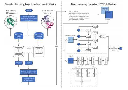
The study of DNA binding proteins (DBPs) is of great importance in the biomedical field and plays a key role in this field. At present, many researchers are working on the prediction and detection of DBPs. Traditional DBP prediction mainly uses machine learning methods. Although these methods can obtain relatively high pre-diction accuracy, they consume large quantities of human effort and material resources. Transfer learning has certain advantages in dealing with such prediction problems. Therefore, in the present study, two features were extracted from a protein sequence, a transfer learning method was used, and two classical transfer learning algorithms were compared to transfer samples and construct data sets. In the final step, DBPs are detected by building a deep learning neural network model in a way that uses attention mechanisms.

| [1] |
L. Wei, W. He, A. Malik, R. Su, L. Cui, B. Manavalan, Computational prediction and interpretation of cell-specific replication origin sites from multiple eukaryotes by exploiting stacking framework, Briefings Bioinf., 22 (2021). https://doi.org/10.1093/bib/bbaa275 doi: 10.1093/bib/bbaa275

|
| [2] |
L. Wei, M. Liao, Y. Gao, R. Ji, Z. He, Q. Zou, Improved and promising identification of human MicroRNAs by incorporating a high-quality negative set, IEEE/ACM Trans. Comput. Biol. Bioinf., 11 (2014), 192–201. https://doi.org/10.1109/TCBB.2013.146 doi: 10.1109/TCBB.2013.146
|
| [3] |
D. H. Ohlendorf, W. F. Anderson, R. G. Fisher, Y. Takeda, B.W. Matthews, The molecular basis of DNA-protein recognition inferred from the structure of cro repressor, Nature, 298 (1982), 718–23. https://doi.org/10.1038/298718a0 doi: 10.1038/298718a0
|
| [4] |
W. H. Hudson, E. A. Ortlund, The structure, function and evolution of proteins that bind DNA and RNA, Nat. Rev. Mol. Cell Biol., 15 (2014), 749–760. https://doi.org/10.1038/nrm3884 doi: 10.1038/nrm3884
|
| [5] |
Y. Ding, J. Tang, F. Guo, Q. Zou, Identification of drug-target interactions via multiple kernel-based triple collaborative matrix factorization, Briefings Bioinf., 23 (2022), bbab582. https://doi.org/10.1093/bib/bbab582 doi: 10.1093/bib/bbab582
|
| [6] |
Y. Ding, J. Tang, F. Guo, Identification of drug–target interactions via dual laplacian regularized least squares with multiple kernel fusion, Knowl.-Based Syst., 204 (2020), 106254. https://doi.org/10.1016/j.knosys.2020.106254 doi: 10.1016/j.knosys.2020.106254
|
| [7] |
Y. Ding, P. Tiwari, Q. Zou, F. Guo, H. M. Pandey, C-loss based Higher-order Fuzzy Inference Systems for identifying DNA N4-methylcytosine Sites, IEEE Trans. Fuzzy Syst., 2022. https://doi.org/10.1109/TFUZZ.2022.3159103 doi: 10.1109/TFUZZ.2022.3159103
|
| [8] |
Y. Ding, W. He, J. Tang, Q. Zou, F. Guo, Laplacian regularized sparse representation based classifier for identifying DNA N4-methylcytosine Sites via L2, 1/2-matrix norm, IEEE/ACM Trans. Comput. Biol. Bioinf., 2021. https://doi.org/10.1109/TCBB.2021.3133309 doi: 10.1109/TCBB.2021.3133309
|
| [9] |
M. Gao, J. Skolnick, DBD-Hunter: a knowledge-based method for the prediction of DNA-protein interactions, Nucleic Acids Res., 36 (2008), 3978–3992. https://doi.org/10.1093/nar/gkn332 doi: 10.1093/nar/gkn332
|
| [10] |
G. Nimrod, M. Schushan, A. Szilagyi, C. Leslie, N. Ben-Tal, iDBPs: a web server for the identification of DNA binding proteins, Bioinformatics, 26 (2010), 692–693. https://doi.org/10.1093/bioinformatics/btq019 doi: 10.1093/bioinformatics/btq019
|
| [11] |
H. Zhao, J. Wang, Y. Zhou, Y. Yang, Predicting DNA-binding proteins and binding residues by complex structure prediction and application to human proteome, PLoS One, (2014), e96694. https://doi.org/10.1371/journal.pone.0096694 doi: 10.1371/journal.pone.0096694
|
| [12] |
M. Remmert, A. Biegert, A. Hauser, J. Soding, HHblits: lightning-fast iterative protein sequence searching by HMM-HMM alignment, Nat. Methods, 9 (2011), 173–175. https://doi.org/10.1038/nmeth.1818 doi: 10.1038/nmeth.1818
|
| [13] |
K. K. Kumar, G. Pugalenthi, P. N. Suganthan, DNA-Prot: identification of DNA binding proteins from protein sequence information using random forest, J. Biomol. Struct. Dyn., 26 (2009), 679–686. https://doi.org/10.1080/07391102.2009.10507281 doi: 10.1080/07391102.2009.10507281
|
| [14] |
B. Liu, S. Wang, X. Wang, DNA binding protein identification by combining pseudo amino acid composition and profile-based protein representation, Sci. Rep., 5 (2015), 15479. https://doi.org/10.1038/srep15479 doi: 10.1038/srep15479
|
| [15] |
K. C. Chou, Some remarks on protein attribute prediction and pseudo amino acid composition, J. Theor. Biol., 273 (2011), 236–247. https://doi.org/10.1016/j.jtbi.2010.12.024 doi: 10.1016/j.jtbi.2010.12.024
|
| [16] |
K. C. Chou, Prediction of protein cellular attributes using pseudo-amino acid composition, Proteins, 43 (2001), 246–255. https://doi.org/10.1002/prot.1035 doi: 10.1002/prot.1035
|
| [17] |
L. Wei, J. Tang, Q. Zou, Local-DPP: an improved DNA-binding protein prediction method by exploring local evolutionary information, Inf. Sci., 384 (2017), 135–144. https://doi.org/10.1016/j.ins.2016.06.026 doi: 10.1016/j.ins.2016.06.026
|
| [18] |
A. Mishra, P. Pokhrel, M. T. Hoque, StackDPPred: a stacking based prediction of DNA-binding protein from sequence, Bioinformatics, 35 (2019), 433–441. https://doi.org/10.1093/bioinformatics/bty653 doi: 10.1093/bioinformatics/bty653
|
| [19] |
L. Nanni, S. Brahnam, Robust ensemble of handcrafted and learned approaches for DNA-binding proteins, Appl. Comput. Inf., 2021. https://doi.org/10.1108/ACI-03-2021-0051 doi: 10.1108/ACI-03-2021-0051
|
| [20] |
Y. H. Qu, H. Yu, X. J. Gong, J. H. Xu, H. S. Lee, On the prediction of DNA-binding proteins only from primary sequences: a deep learning approach, PLoS One, (2017), e0188129. https://doi.org/10.1371/journal.pone.0188129 doi: 10.1371/journal.pone.0188129
|
| [21] |
S. Shadab, T. A. Khan, N. A. Neezi, S. Adilina, S. Shatabda, DeepDBP: deep neural networks for identification of DNA-binding proteins, Inf. Med. Unlocked, 19 (2020), 100318. https://doi.org/10.1016/j.imu.2020.100318 doi: 10.1016/j.imu.2020.100318
|
| [22] |
S. Ahmad, A. Sarai, PSSM-based prediction of DNA binding sites in proteins, BMC Bioinf., 6 (2005), 33. https://doi.org/10.1186/1471-2105-6-33 doi: 10.1186/1471-2105-6-33
|
| [23] |
J. Zhang, Q. Chen, B. Liu, DeepDRBP-2L: a new genome annotation predictor for identifying DNA-binding proteins and RNA-binding proteins using convolutional neural network and long short-term memory, IEEE/ACM Trans. Comput. Biol. Bioinf., 18 (2021), 1451–1463. https://doi.org/10.1109/TCBB.2019.2952338 doi: 10.1109/TCBB.2019.2952338
|
| [24] |
J. Zhang, Q. Chen, B. Liu, iDRBP_MMC: identifying DNA-binding proteins and RNA-binding proteins based on multi-label learning model and motif-based convolutional neural network, J. Mol. Biol., 432 (2020), 5860–5875. https://doi.org/10.1016/j.jmb.2020.09.008 doi: 10.1016/j.jmb.2020.09.008
|
| [25] |
G. Li, X. Du, X. Li, L. Zou, G. Zhang, Z. Wu, Prediction of DNA binding proteins using local features and long-term dependencies with primary sequences based on deep learning, PeerJ, 9 (2021), e11262. https://doi.org/10.7717/peerj.11262 doi: 10.7717/peerj.11262
|
| [26] |
K. Greff, R. K. Srivastava, J. Koutnik, B. R. Steunebrink, J. Schmidhuber, LSTM: a search space odyssey, IEEE Trans. Neural Networks Learn. Syst., 28 (2017), 2222–2232. https://doi.org/10.1109/TNNLS.2016.2582924 doi: 10.1109/TNNLS.2016.2582924
|
| [27] |
T. Roska, L. O. Chua, The CNN universal machine: an analogic array computer, IEEE Trans. Circuits Syst. II, 40 (1993), 163–173. https://doi.org/10.1109/82.222815 doi: 10.1109/82.222815
|
| [28] | C. Szegedy, S. Ioffe, V. Vanhoucke, A. A. Alemi, Inception-v4, inception-resnet and the impact of residual connections on learning, in Proceedings of the Thirty-First AAAI Conference on Artificial Intelligence, (2017), 4278–4284. Available from: https://dl.acm.org/doi/10.5555/3298023.3298188. |
| [29] |
B. Liu, J. Xu, X. Lan, R. Xu, J. Zhou, X. Wang, et al., iDNA-Prot|dis: identifying DNA-binding proteins by incorporating amino acid distance-pairs and reduced alphabet profile into the general pseudo amino acid composition, PLoS One, (2014), e106691. https://doi.org/10.1371/journal.pone.0106691 doi: 10.1371/journal.pone.0106691
|
| [30] |
Y. Wang, Y. Ding, F. Guo, L. Wei, J. Tang, Improved detection of DNA-binding proteins via compression technology on PSSM information, PLoS One, (2017), e0185587. https://doi.org/10.1371/journal.pone.0185587 doi: 10.1371/journal.pone.0185587
|
| [31] | R. Caruana, A. Niculescu-Mizil, An empirical comparison of supervised learning algorithms, in Proceedings of the 23rd International Conference on Machine Learning, (2006), 161–168. https://doi.org/10.1145/1143844.1143865 |
| [32] |
K. Weiss, T. M. Khoshgoftaar, D. Wang, A survey of transfer learning, J. Big Data, 3 (2016), 9. https://doi.org/10.1186/s40537-016-0043-6 doi: 10.1186/s40537-016-0043-6
|
| [33] |
S. J. Pan, Q. Yang, A survey on transfer learning, IEEE Trans. Knowl. Data Eng., 22 (2010), 1345–1359. https://doi.org/10.1109/TKDE.2009.191 doi: 10.1109/TKDE.2009.191
|
| [34] | M. Oquab, L. Bottou, I. Laptev, J. Sivic, Learning and transferring mid-level image representations using convolutional neural networks, in 2014 IEEE Conference on Computer Vision and Pattern Recognition, (2014), 1717–1724. https://doi.org/10.1109/CVPR.2014.222 |
| [35] | W. Dai, Q. Yang, G. Xue, Y. Yu, Boosting for transfer learning, Machine Learning, inProceedings of the 24th International Conference on Machine Learning, (2007), 193–200. https://doi.org/10.1145/1273496.1273521 |
| [36] | S. R. Bowman, L. Vilnis, O. Vinyals, A. M. Dai, R. Jozefowicz, S. Bengio, Generating sentences from a continuous space, in Proceedings of the 20th SIGNLL Conference on Computational Natural Language Learning, (2016), 10–21. https://doi.org/10.18653/v1/K16-1002 |
| [37] | E. Tzeng, J. Hoffman, N. Zhang, K. Saenko, T. Darrell, Deep domain confusion: Maximizing for domain invariance, preprient, arXiv: 1412.3474. |
| [38] | H. Yan, Y. Ding, P. Li, Q. Wang, Y. Xu, W. Zuo, Mind the class weight bias: weighted maximum mean discrepancy for unsupervised domain adaptation, in 2017 IEEE Conference on Computer Vision and Pattern Recognition (CVPR), (2017), 945–954. https://doi.org/10.1109/CVPR.2017.107 |
| [39] | W. Qin, X. Cui, C. A. Yuan, X. Qin, L. Shang, Z. K. Huang, et al., Flower species recognition system combining object detection and attention mechanism, in International Conference on Intelligent Computing, Springer, 2019. https://doi.org/10.1007/978-3-030-26766-7_1 |
| [40] | K. Cho, B. V. Merriënboer, C. Gulcehre, D. Bahdanau, F. Bougares, H. Schwenk, et al., Learning phrase representations using RNN encoder-decoder for statistical machine translation, in Proceedings of the 2014 Conference on Empirical Methods in Natural Language Processing (EMNLP), (2014), 1724–1734. https://doi.org/10.3115/v1/D14-1179 |
| [41] | T. Mikolov, S. Kombrink, L. Burget, J. Černocký, S. Khudanpur, Extensions of recurrent neural network language model, in 2011 IEEE International Conference on Acoustics, Speech and Signal Processing (ICASSP), (2011), 5528–5531. https://doi.org/10.1109/ICASSP.2011.5947611 |
| [42] |
L. Wei, C. Zhou, H. Chen, J. Song, R. Su, ACPred-FL: a sequence-based predictor using effective feature representation to improve the prediction of anti-cancer peptides, Bioinformatics, 34 (2018), 4007–4016. https://doi.org/10.1093/bioinformatics/bty451 doi: 10.1093/bioinformatics/bty451
|
| [43] |
Y. Ding, J. Tang, F. Guo, Protein crystallization identification via fuzzy model on linear neighborhood representation, IEEE/ACM Trans. Comput. Biol. Bioinf., 18 (2021), 1986–1995. https://doi.org/10.1109/TCBB.2019.2954826 doi: 10.1109/TCBB.2019.2954826
|
| [44] |
Y. Ding, J. Tang, F. Guo, Human protein subcellular localization identification via fuzzy model on kernelized neighborhood representation, Appl. Soft Comput., 96 (2020), 106596. https://doi.org/10.1016/j.asoc.2020.106596 doi: 10.1016/j.asoc.2020.106596
|
| [45] | S. K. Knapp, Accelerate FPGA macros with one-hot approach, Electron. Des., 1990. |
| [46] |
J. Soding, Protein homology detection by HMM-HMM comparison, Bioinformatics, 21 (2005), 951–960. https://doi.org/10.1093/bioinformatics/bti125 doi: 10.1093/bioinformatics/bti125
|
| [47] | K. He, X. Zhang, S. Ren, J. Sun, Deep residual learning for image recognition, in 2016 IEEE Conference on Computer Vision and Pattern Recognition (CVPR), (2016), 770–778. https://doi.org/10.1109/CVPR.2016.90 |
| [48] | V. Nair, G. E. Hinton, Rectified linear units improve restricted boltzmann machines, in Proceedings of the 27th International Conference on International Conference on Machine Learning, (2010), 807–814. Available from: https://dl.acm.org/doi/10.5555/3104322.3104425. |
| [49] | A. Paszke, S. Gross, S. Chintala, G. Chanan, E. Yang, Z. DeVito, et al., Automatic differentiation in pytorch, 2017. Available from: https://paperswithcode.com/paper/automatic-differentiation-in-pytorch. |
| [50] | D. P. Kingma, J. Ba, Adam: a method for stochastic optimization, CoRR, 2015. Available from: https://www.semanticscholar.org/paper/Adam%3A-A-Method-for-Stochastic-Optimization-Kingma-Ba/a6cb366736791bcccc5c8639de5a8f9636bf87e8. |
| [51] |
W. Lou, X. Wang, F. Chen, Y. Chen, B. Jiang, H. Zhang, Sequence based prediction of DNA-binding proteins based on hybrid feature selection using random forest and Gaussian naive Bayes, PLoS One, (2014), e86703. https://doi.org/10.1371/journal.pone.0086703 doi: 10.1371/journal.pone.0086703
|
| [52] |
P. W. Rose, A. Prlic, C. Bi, W. F. Bluhm, C. H. Christie, S. Dutta, et al., The RCSB Protein Data Bank: views of structural biology for basic and applied research and education, Nucleic Acids Res., 43 (2015), D345–D356. https://doi.org/10.1093/nar/gku1214 doi: 10.1093/nar/gku1214
|
| [53] |
X. Du, Y. Diao, H. Liu, S. Li, MsDBP: Exploring DNA-binding proteins by integrating multiscale sequence information via Chou's five-step rule, J. Proteome Res., 18 (2019), 3119–3132. https://doi.org/10.1021/acs.jproteome.9b00226 doi: 10.1021/acs.jproteome.9b00226
|


Figures(4) / Tables(5)

Jun Yan, Tengsheng Jiang, Junkai Liu, Yaoyao Lu, Shixuan Guan, Haiou Li, Hongjie Wu, Yijie Ding. DNA-binding protein prediction based on deep transfer learning[J]. Mathematical Biosciences and Engineering, 2022, 19(8): 7719-7736. doi: 10.3934/mbe.2022362


 DownLoad: