Comparison of exact and approximate approaches to UAVs mission contingency planning in dynamic environments

Grzegorz Radzki; Grzegorz Bocewicz; Jaroslaw Wikarek; Peter Nielsen; Zbigniew Banaszak; Grzegorz Radzki; Grzegorz Bocewicz; Jaroslaw Wikarek; Peter Nielsen; Zbigniew Banaszak

doi:10.3934/mbe.2022335

Mathematical Biosciences and Engineering

2022, Volume 19, Issue 7: 7091-7121. doi: 10.3934/mbe.2022335

Previous Article Next Article

Research article Special Issues

Comparison of exact and approximate approaches to UAVs mission contingency planning in dynamic environments

1.
Faculty of Electronics and Computer Science, Koszalin University of Technology, Poland
2.
Department of Information Systems, Kielce University of Technology, Kielce, Poland
3.
Department of Materials and Production, Aalborg University, Denmark

Academic Editor: Fernando De la Prieta

Received: 25 February 2022 Revised: 30 April 2022 Accepted: 05 May 2022 Published: 13 May 2022

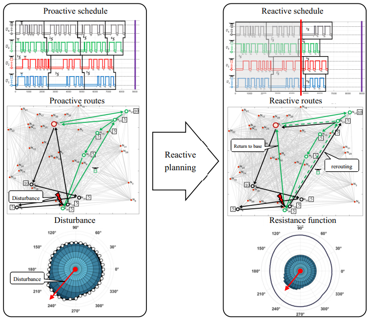
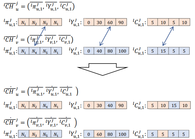
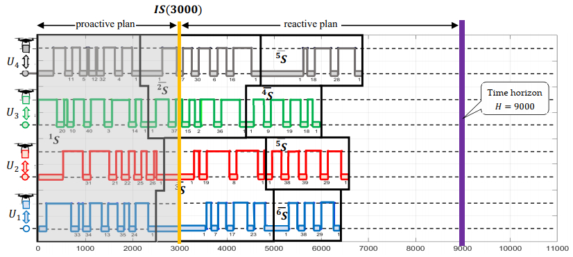
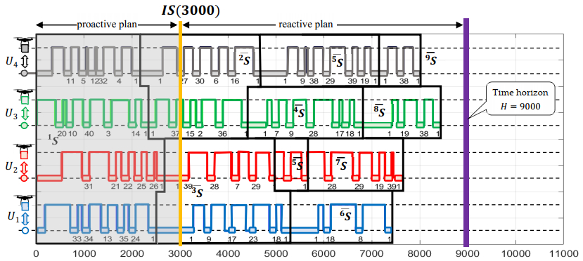
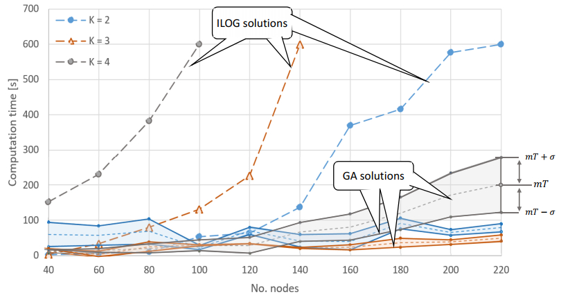
This paper presents a novel approach to the joint proactive and reactive planning of deliveries by an unmanned aerial vehicle (UAV) fleet. We develop a receding horizon-based approach to contingency planning for the UAV fleet's mission. We considered the delivery of goods to spatially dispersed customers, over an assumed time horizon. In order to take into account forecasted weather changes that affect the energy consumption of UAVs and limit their range, we propose a set of reaction rules that can be encountered during delivery in a highly dynamic and unpredictable environment. These rules are used in the course of designing the contingency plans related to the need to implement an emergency return of the UAV to the base or handling of ad hoc ordered deliveries. Due to the nonlinearity of the environment's characteristics, both constraint programming and genetic algorithm paradigms have been implemented. Because of the NP-difficult nature of the considered planning problem, conditions have been developed that allow for the acceleration of calculations. The multiple computer experiments carried out allow for comparison representatives of the approximate and exact methods so as to judge which approach is faster for which size of the selected instance of the UAV mission planning problem.
- contingency planning,
- UAV fleet mission,
- weather changes,
- declarative modeling,
- genetic algorithm
Citation: Grzegorz Radzki, Grzegorz Bocewicz, Jaroslaw Wikarek, Peter Nielsen, Zbigniew Banaszak. Comparison of exact and approximate approaches to UAVs mission contingency planning in dynamic environments[J]. Mathematical Biosciences and Engineering, 2022, 19(7): 7091-7121. doi: 10.3934/mbe.2022335

Related Papers:

Abstract

This paper presents a novel approach to the joint proactive and reactive planning of deliveries by an unmanned aerial vehicle (UAV) fleet. We develop a receding horizon-based approach to contingency planning for the UAV fleet's mission. We considered the delivery of goods to spatially dispersed customers, over an assumed time horizon. In order to take into account forecasted weather changes that affect the energy consumption of UAVs and limit their range, we propose a set of reaction rules that can be encountered during delivery in a highly dynamic and unpredictable environment. These rules are used in the course of designing the contingency plans related to the need to implement an emergency return of the UAV to the base or handling of ad hoc ordered deliveries. Due to the nonlinearity of the environment's characteristics, both constraint programming and genetic algorithm paradigms have been implemented. Because of the NP-difficult nature of the considered planning problem, conditions have been developed that allow for the acceleration of calculations. The multiple computer experiments carried out allow for comparison representatives of the approximate and exact methods so as to judge which approach is faster for which size of the selected instance of the UAV mission planning problem.

References

[1]	K. Dorling, J. Heinrichs, G. G. Messier, S. Magierowski, Vehicle routing problems for drone delivery, IEEE Trans. Syst. Man Cybern. Syst., 47 (2017), 70–85. https://doi.org/10.1109/TSMC.2016.2582745 doi: 10.1109/TSMC.2016.2582745
[2]	J. J. Enright, E. Frazzoli, M. Pavone, S. Ketan, UAV routing and coordination in stochastic, dynamic environments, in Handbook of Unmanned Aerial Vehicles (eds. K. P. Valavanis and G. J. Vachtsevanos), Springer, Dordrecht, (2015), 2079–2109. https://doi.org/10.1007/978-90-481-9707-1_28
[3]	Y. Khosiawan, A. Khalfay, I. Nielsen, Scheduling unmanned aerial vehicle and automated guided vehicle operations in an indoor manufacturing environment using differential evolution-fused particle swarm optimization, Int. J. Adv. Rob. Syst., 15 (2018). https://doi.org/10.1177/1729881417754145 doi: 10.1177/1729881417754145
[4]	S. M. Patella, G. Grazieschi, V. Gatta, E. Marcucci, S. Carrese, The adoption of green vehicles in last mile logistics: a systematic review, Sustainability, 13 (2021), 6. https://doi.org/10.3390/su13010006 doi: 10.3390/su13010006
[5]	I. Sung, P. Nielsen, Zoning a service area of unmanned aerial vehicles for package delivery services, J. Intell. Rob. Syst., 97 (2020), 719–731. https://doi.org/10.1007/s10846-019-01045-7 doi: 10.1007/s10846-019-01045-7
[6]	A. Thibbotuwawa, G. Bocewicz, G. Radzki, P. Nielsen, Z. Banaszak, UAV mission planning resistant to weather uncertainty, Sensors, 20 (2020), 515. https://doi.org/10.3390/s20020515 doi: 10.3390/s20020515
[7]	A. Troudi, S. A. Addouche, S. Dellagi, A. E. Mhamedi, Sizing of the drone delivery fleet considering energy autonomy, Sustainability, 10 (2018), 3344. https://doi.org/10.3390/su10093344 doi: 10.3390/su10093344
[8]	A. Thibbotuwawa, P. Nielsen, B. Zbigniew, G. Bocewicz, Energy consumption in unmanned aerial vehicles: A review of energy consumption models and their relation to the UAV routing, in International Conference on Information Systems Architecture and Technology, (2018), 173–184. https://doi.org/10.1007/978-3-319-99996-8_16
[9]	J. Hall, D. Anderson, Reactive route selection from pre-calculated trajectories—application to micro-UAV path planning, Aeronaut. J., 115 (2011), 635–640. https://doi.org/10.1017/S0001924000006321 doi: 10.1017/S0001924000006321
[10]	R. Shirani, M. St-Hilaire, T. Kunz, Y. Zhou, J. Li, L. Lamont, On the delay of reactive-greedy-reactive routing in unmanned aeronautical ad-hoc network, Procedia Comput. Sci., 10 (2012), 535–542. https://doi.org/10.1016/j.procs.2012.06.068 doi: 10.1016/j.procs.2012.06.068
[11]	W. Bożejko, A. Gnatowski, J. Pempera, M. Wodecki, Parallel tabu search for the cyclic job shop scheduling problem, Comput. Ind. Eng., 113 (2017), 512–524. https://doi.org/10.1016/j.cie.2017.09.042 doi: 10.1016/j.cie.2017.09.042
[12]	B. N. Coelho, V. N. Coelho, I. M. Coelho, L. S. Ochi, R. H. Koochaksaraei, D. Zuidema, et al., A multi-objective green UAV routing problem, Comput. Oper. Res., 88 (2017), 306–315. https://doi.org/10.1016/j.cor.2017.04.011 doi: 10.1016/j.cor.2017.04.011
[13]	M. A. R. Estrada, A. Ndoma, The uses of unmanned aerial vehicles—UAV's-(or drones) in social logistic: natural disasters response and humanitarian relief aid, Procedia Comput. Sci., 149 (2019), 375–383. https://doi.org/10.1016/j.procs.2019.01.151 doi: 10.1016/j.procs.2019.01.151
[14]	P. Golinska, M. Hajdul, Multi-agent coordination mechanism of virtual supply chain, in KES International Symposium on Agent and Multi-Agent Systems: Technologies and Applications, Springer, Berlin, (2011), 620–629. https://doi.org/10.1007/978-3-642-22000-5_64
[15]	P. Golinska, M. Hajdul, Virtual logistics clusters—IT support for integration, in Asian Conference on Intelligent Information and Database System, Springer, Berlin, (2012), 449–458. https://doi.org/10.1007/978-3-642-28487-8_47
[16]	M. Lohatepanont, C. Barnhart, Airline schedule planning: integrated models and algorithms for schedule design and fleet assignment, Transp. Sci., 38 (2004), 19–32. https://doi.org/10.1287/trsc.1030.0026 doi: 10.1287/trsc.1030.0026
[17]	P. Sitek, J. Wikarek, A multi-level approach to ubiquitous modeling and solving constraints in combinatorial optimization problems in production and distribution, Appl. Intell., 48 (2018), 1344–1367. https://doi.org/10.1007/s10489-017-1107-9 doi: 10.1007/s10489-017-1107-9
[18]	A. Thibbotuwawa, G. Bocewicz, B. Zbigniew, P. Nielsen, A solution approach for UAV fleet mission planning in changing weather conditions, Appl. Sci., 9 (2019), 3972. https://doi.org/10.3390/app9193972 doi: 10.3390/app9193972
[19]	P. Traverso, E. Giunchiglia, L. Spalazzi, F. Giunchiglia, Formal theories for reactive planning systems: some considerations raised from an experimental application, in AAAI Technical Report WS-96-07, 1996.
[20]	O. Oubbati, A. Lakas, M. Güneş, F. Zhou, M. B. Yagoubi, UAV-assisted reactive routing for urban VANETs, in Proceedings of the Symposium on Applied Computing, (2017), 651–653. https://doi.org/10.1145/3019612.3019904
[21]	O. S. Oubbati, N. Chaib, A. Lakas, S. Bitam, P. Lorenz, U2RV: UAV-assisted reactive routing protocol for VANETs, Int. J. Commun. Syst., 33 (2020), e4104. https://doi.org/10.1002/dac.4104 doi: 10.1002/dac.4104
[22]	G. Radzki, P. Nielsen, G. Bocewicz, Z. Banaszak, A proactive approach to resistant UAV mission planning, in Conference on Automation, Springer, Cham, (2020), 112–124. https://doi.org/10.1007/978-3-030-40971-5_11
[23]	M. Relich, G. Bocewicz, K. B. Rostek, Z. Banaszak, A declarative approach to new product development project prototyping, IEEE Intell. Syst., 36 (2020), 88–95. https://doi.org/10.1109/MIS.2020.3030481 doi: 10.1109/MIS.2020.3030481
[24]	A. Thibbotuwawa, G. Bocewicz, P. Nielsen, Z. Banaszak, Unmanned aerial vehicle routing problems: a literature review, Appl. Sci., 10 (2020), 4504. https://doi.org/10.3390/app10134504 doi: 10.3390/app10134504
[25]	T. Elmokadem, A. V. Savkin, A hybrid approach for autonomous collision-free UAV navigation in 3D partially unknown dynamic environments, Drones, 5 (2021), 57. https://doi.org/10.3390/drones5030057 doi: 10.3390/drones5030057
[26]	M. Halat, Ö. Özkan, The optimization of UAV routing problem with a genetic algorithm to observe the damages of possible Istanbul earthquake, Pamukkale Üniversitesi Mühendislik Bilimleri Dergisi, 27 (2021), 187–198. https://doi.org/10.5505/pajes.2020.75725 doi: 10.5505/pajes.2020.75725
[27]	K. E. C. Booth, Constraint Programming Approaches to Electric Vehicle and Robot Routing Problems, Ph. D thesis, University of Toronto, 2021.
[28]	M. A. Russell, G. B. Lamont, A genetic algorithm for unmanned aerial vehicle routing, in Proceedings of the 7th Annual Conference on Genetic and Evolutionary Computation, (2005), 1523–1530. https://doi.org/10.1145/1068009.1068249
[29]	J. E. Baculi, C. A. Ippolito, Onboard decision-making for nominal and contingency sUAS flight, in AIAA Scitech 2019 Forum, 2019. https://doi.org//10.2514/6.2019-1457
[30]	S. Bhargava, A note on evolutionary algorithms and its applications, Adults Learning Math., 8 (2013), 31–45.
[31]	C. Guettier, F. Lucas, A constraint-based approach for planning unmanned aerial vehicle activities, Knowl. Eng. Rev., 31 (2016), 486–497. https://doi.org/10.1017/S0269888916000291 doi: 10.1017/S0269888916000291
[32]	I. K. Nikolos, E. S. Zografos, A. N. Brintaki, UAV path planning using evolutionary algorithms, in Innovations in Intelligent Machines-1 (eds. J. S. Chahl, L. C. Jain, A. Mizutani, and M. Sato-Ilic), Springer, Berlin, (2007), 77–111. https://doi.org/10.1007/978-3-540-72696-8_4
[33]	G. Radzki, M. Relich, G. Bocewicz, Z. Banaszak, Declarative approach to UAVs mission contingency planning in dynamic environments, in International Symposium on Distributed Computing and Artificial Intelligence, Springer, 2021. https://doi.org/10.1007/978-3-030-86887-1_1
[34]	Z. Fu, J. Yu, G. Xie, Y. Chen, Y. Mao, A heuristic evolutionary algorithm of UAV path planning, Wireless Commun. Mobile Comput., 2018 (2018). https://doi.org/10.1155/2018/2851964 doi: 10.1155/2018/2851964
[35]	R. Nagasawa, E. Mas, L. Moya, Model-based analysis of multi-UAV path planning for surveying postdisaster building damage, Sci. Rep., 11 (2021), 1–14. https://doi.org/10.1038/s41598-021-97804-4 doi: 10.1038/s41598-021-97804-4
[36]	B. B. K. Ayawli, R. Chellali, A. Y. Appiah, F. Kyeremeh, An overview of nature-inspired, conventional, and hybrid methods of autonomous vehicle path planning, J. Adv. Transp., 2018 (2018). https://doi.org/10.1155/2018/8269698 doi: 10.1155/2018/8269698
[37]	J. Hu, H. Wu, R. Zhan, M. Rafik, X. Zhou, Self-organized search-attack mission planning for UAV swarm based on wolf pack hunting behavior, J. Syst. Eng. Electron., 32 (2021), 1463–1476. https://doi.org/10.23919/JSEE.2021.000124 doi: 10.23919/JSEE.2021.000124
[38]	N. Lin, J. Tang, X. Li, L. Zhao, A novel improved bat algorithm in UAV path planning, J. Comput. Mater. Contin., 61 (2019), 323–344. https://doi.org/10.32604/cmc.2019.05674 doi: 10.32604/cmc.2019.05674
[39]	V. Rodríguez-Fernández, H. D. Menéndez, D. Camacho, Design and development of a lightweight multi-UAV simulator, in 2015 IEEE 2nd International Conference on Cybernetics (CYBCONF), (2015), 255–260. https://doi.org/10.1109/CYBConf.2015.7175942
[40]	J. C. Rubio, J. Vagners, R. Rysdyk, Adaptive path planning for autonomous UAV oceanic search missions, in AIAA 1st Intelligent Systems Technical Conference, 2004. https://doi.org/10.2514/6.2004-6228
[41]	P. Calégari, G. Coray, A. Hertz, D. Kobler, P. Kuonen, A taxonomy of evolutionary algorithms in combinatorial optimization, J. Heuristics, 5 (1999), 145–158. https://doi.org/10.1023/A:1009625526657 doi: 10.1023/A:1009625526657
[42]	A. Slowik, H. Kwasnicka, Evolutionary algorithms and their applications to engineering problems, Neural Comput. Appl., 32 (2020), 12363–12379. https://doi.org/10.1007/s00521-020-04832-8 doi: 10.1007/s00521-020-04832-8
[43]	J. Stork, A. E. Eiben, T. Bartz-Beielstein, A new taxonomy of global optimization algorithms, Nat. Comput., 2020 (2020), 1–24. https://doi.org/10.1007/s11047-020-09820-4 doi: 10.1007/s11047-020-09820-4

Reader Comments

Your name:*

Email:*
© 2022 the Author(s), licensee AIMS Press. This is an open access article distributed under the terms of the Creative Commons Attribution License (http://creativecommons.org/licenses/by/4.0)