Crude oil prices and volatility prediction by a hybrid model based on kernel extreme learning machine

Hongli Niu; Yazhi Zhao; Hongli Niu; Yazhi Zhao

doi:10.3934/mbe.2021402

Mathematical Biosciences and Engineering

2021, Volume 18, Issue 6: 8096-8122. doi: 10.3934/mbe.2021402

Previous Article Next Article

Research article Special Issues

Crude oil prices and volatility prediction by a hybrid model based on kernel extreme learning machine

Hongli Niu ^,,
Yazhi Zhao

School of Economics and Management, University of Science and Technology Beijing, Beijing 100083, China

Academic Editor: Kuen-Suan Chen

Received: 13 August 2021 Accepted: 15 September 2021 Published: 17 September 2021

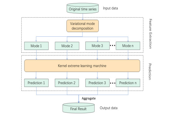
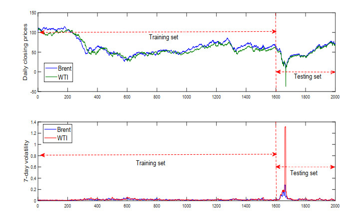
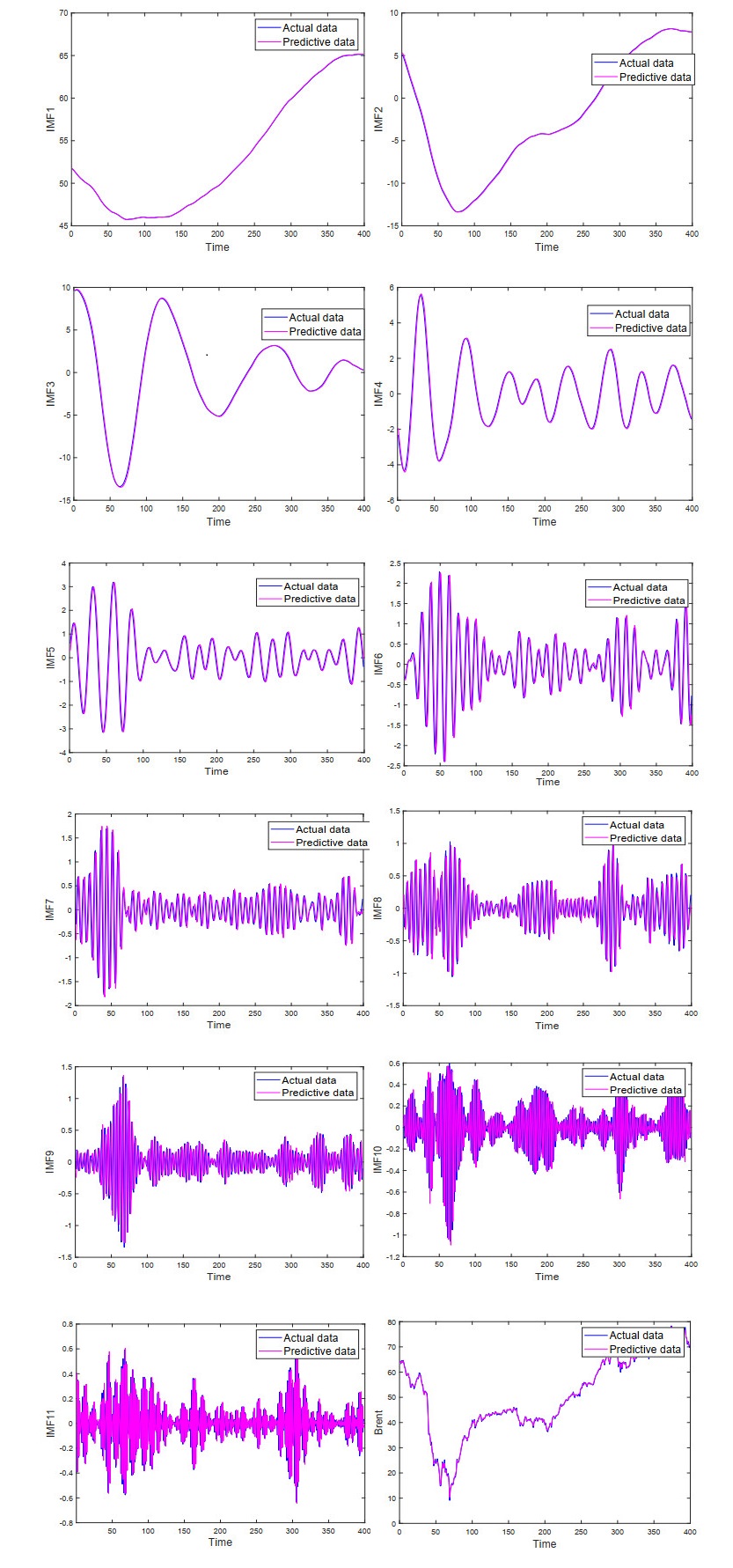
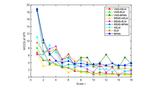
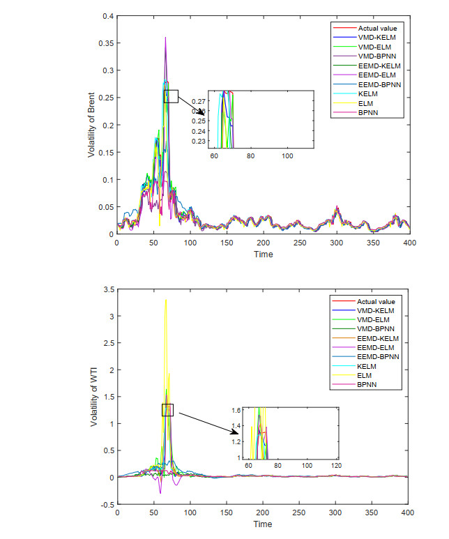
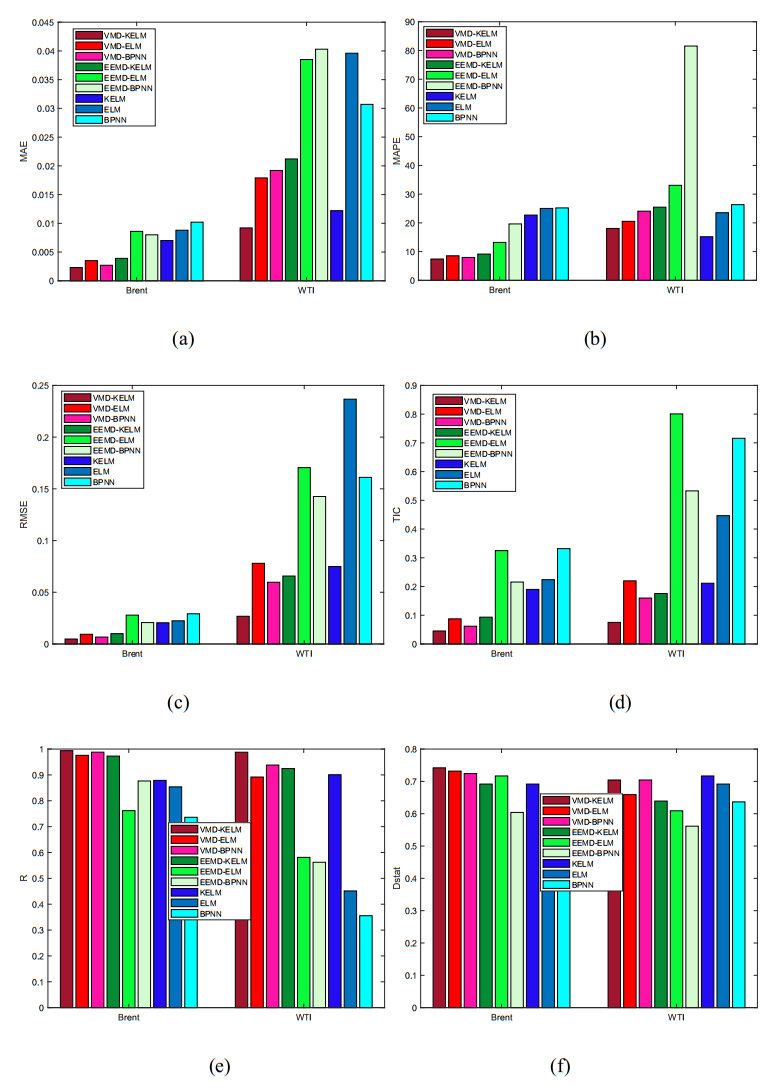
In view of the important position of crude oil in the national economy and its contribution to various economic sectors, crude oil price and volatility prediction have become an increasingly hot issue that is concerned by practitioners and researchers. In this paper, a new hybrid forecasting model based on variational mode decomposition (VMD) and kernel extreme learning machine (KELM) is proposed to forecast the daily prices and 7-day volatility of Brent and WTI crude oil. The KELM has the advantage of less time consuming and lower parameter-sensitivity, thus showing fine prediction ability. The effectiveness of VMD-KELM model is verified by a comparative study with other hybrid models and their single models. Except various commonly used evaluation criteria, a recently-developed multi-scale composite complexity synchronization (MCCS) statistic is also utilized to evaluate the synchrony degree between the predictive and the actual values. The empirical results verify that 1) KELM model holds better performance than ELM and BP in crude oil and volatility forecasting; 2) VMD-based model outperforms the EEMD-based model; 3) The developed VMD-KELM model exhibits great superiority compared with other popular models not only for crude oil price, but also for volatility prediction.
- crude oil prediction,
- variational mode decomposition,
- kernel extreme learning machine,
- hybrid model,
- volatility
Citation: Hongli Niu, Yazhi Zhao. Crude oil prices and volatility prediction by a hybrid model based on kernel extreme learning machine[J]. Mathematical Biosciences and Engineering, 2021, 18(6): 8096-8122. doi: 10.3934/mbe.2021402

Related Papers:

Abstract

In view of the important position of crude oil in the national economy and its contribution to various economic sectors, crude oil price and volatility prediction have become an increasingly hot issue that is concerned by practitioners and researchers. In this paper, a new hybrid forecasting model based on variational mode decomposition (VMD) and kernel extreme learning machine (KELM) is proposed to forecast the daily prices and 7-day volatility of Brent and WTI crude oil. The KELM has the advantage of less time consuming and lower parameter-sensitivity, thus showing fine prediction ability. The effectiveness of VMD-KELM model is verified by a comparative study with other hybrid models and their single models. Except various commonly used evaluation criteria, a recently-developed multi-scale composite complexity synchronization (MCCS) statistic is also utilized to evaluate the synchrony degree between the predictive and the actual values. The empirical results verify that 1) KELM model holds better performance than ELM and BP in crude oil and volatility forecasting; 2) VMD-based model outperforms the EEMD-based model; 3) The developed VMD-KELM model exhibits great superiority compared with other popular models not only for crude oil price, but also for volatility prediction.

References

[1]	G. Wu, Y. Z. Zhang, Does China factor matter? An econometric analysis of international crude oil prices, Energy Policy, 72 (2014), 78-86. doi: 10.1016/j.enpol.2014.04.026
[2]	Y. Zhao, J. P. Li, L. Yu, A deep learning ensemble approach for crude oil price forecasting, Energy Econ., 66 (2017), 9-16. doi: 10.1016/j.eneco.2017.05.023
[3]	L. Yu, Y. Zhao, L. Tang, Ensemble forecasting for complex time series using sparse, representation and neural networks, J. Forecast., 36 (2017).
[4]	M. Monge, L. A. Gil-Alana, P. D. G. Fernando, Crude oil price behaviour before and after military conflicts and geopolitical events, Energy, 120 (2017), 79-91. doi: 10.1016/j.energy.2016.12.102
[5]	D. W. Jones, P. N. Leiby, I. K. Paik, Oil price shocks and the macroeconomy: what has been learned since 1996, Energy J., 25 (2004), 1-32.
[6]	S. Lahmiri, Comparing variational and empirical mode decomposition in forecasting day-ahead energy prices, IEEE Syst. J., 11 (2017), 1907-1910. doi: 10.1109/JSYST.2015.2487339
[7]	S. R. Li, Y. L. Ge, Crude oil price prediction based on a dynamic correcting support vector regression machine, Abstr. Appl. Anal., 2013 (2013), 666-686.
[8]	L. Yu, W. Dai, L. Tang, J. Wu, A hybrid grid-GA-based LSSVR learning paradigm for crude oil price forecasting, Neural Comput. Appl., 27 (2016), 2193-2215. doi: 10.1007/s00521-015-1999-4
[9]	G. B. Huang, Q. Y. Zhu, C.K. Siew, Extreme learning machine: a new learning scheme of feed forward neural networks, in 2004 IEEE international joint conference on neural networks, 2 (2004), 985-990.
[10]	G. B. Huang, H. Zhou, X. Ding, R. Zhang, Extreme learning machine for regression and multiclass classification, IEEE Trans. Syst., Man, Cybern., 42 (2012), 513-529. doi: 10.1109/TSMCB.2011.2168604
[11]	L. Tang, Y. Wu, L. Yu, A randomized-algorithm-based decomposition-ensemble learning methodology for energy price forecasting, Energy, 157 (2018), 526-538. doi: 10.1016/j.energy.2018.05.146
[12]	L. Zhang, P. Suganthan, A survey of randomized algorithms for training neural networks, Inf. Sci., 364 (2016), 146-155.
[13]	G. B. Huang, An insight into extreme learning machines: random neurons, random features and kernels, Cognit. Comput., 6 (2014), 376-390.
[14]	S. Ding, Y. Zhang, X. Xu, L. Bao, A novel extreme learning machine based on hybrid kernel function, J. Comput. Phys., 8 (2013), 2110-2117.
[15]	M. Pal, A. E. Maxwell, T. A. Warner, Kernel-based extreme learning machine for remote sensing image classification, Remote Sens. Lett., 4 (2013), 853-862. doi: 10.1080/2150704X.2013.805279
[16]	C. Chen, W. Li, H. Su, K. Liu, Spectral-spatial classification of hyperspectral image based on kernel extreme learning machine, Remote Sens., 6 (2014), 5795-5814. doi: 10.3390/rs6065795
[17]	W. Y. Deng, Q. H. Zheng, Z. M. Wang, Cross-person activity recognition using reduced kernel extreme learning machine, Neural Networks, 53 (2014), 1-7. doi: 10.1016/j.neunet.2014.01.008
[18]	S. Shamshirband, K. Mohammadi, H. L. Chen, G. N. Samy, D. Petković, C. Ma, Daily global solar radiation prediction from air temperatures using kernel extreme learning machine: A case study for Iran, J. Atmos. Sol.-Terr. Phys., 134 (2015), 109-117. doi: 10.1016/j.jastp.2015.09.014
[19]	I. Majumder, P. K. Dash, R. Biso, Variational mode decomposition based low rank robust kernel extreme learning machine for solar irradiation forecasting, Energy Convers. Manage., 171 (2018), 787-780. doi: 10.1016/j.enconman.2018.06.021
[20]	R. Jammazi, C. Aloui, Crude oil price forecasting: Experimental evidence from wavelet decomposition and neural network modeling, Energy Econ., 34 (2012), 828-841. doi: 10.1016/j.eneco.2011.07.018
[21]	K. Dragomiretskiy, D. Zosso, Variational mode decomposition, IEEE Trans. Signal Process., 62 (2014), 531-544.
[22]	J.C. Li, S.W. Zhu, Q.Q. Wu, Monthly crude oil spot price forecasting using variational mode decomposition, Energy Econ., 83 (2019), 240-253. doi: 10.1016/j.eneco.2019.07.009
[23]	R. Bisoi, P. K. Dash, S. P. Mishra, Modes decomposition method in fusion with robust random vector functional link network for crude oil price forecasting, Appl. Soft Comput. J., 80 (2019), 475-493. doi: 10.1016/j.asoc.2019.04.026
[24]	H. Niu, K. Xu, W. Wang, A hybrid stock price index forecasting model based on variational mode decomposition and LSTM network, Appl. Intell., 50 (2020), 4296-4309. doi: 10.1007/s10489-020-01814-0
[25]	L. Huang, J. Wang, Global crude oil price prediction and synchronization based accuracy evaluation using random wavelet neural network, Energy, 151 (2018), 875-888.
[26]	K. Kanjilal, S. Ghosh, Dynamics of crude oil and gold price post 2008 global financial crisis-New evidence from threshold vector error-correction model, Resour. Policy, 52 (2017), 358-365. doi: 10.1016/j.resourpol.2017.04.001
[27]	L. Lin, Y. Jiang, H. Xiao, Z. Zhou, Crude oil price forecasting based on a novel hybrid long memory GARCH-M and wavelet analysis model, Phys. A, 543 (2020), 123532. doi: 10.1016/j.physa.2019.123532
[28]	Y. Xiang, X. H. Zhuang, Application of ARIMA model in short-term prediction of international crude oil price, Adv. Mater. Res., 798-799 (2013), 979-982.
[29]	M. Marchese, L. Kyriakou, M. Tamvakis, F. D. Iorio, Forecasting crude oil and refined products volatilities and correlations: New evidence from fractionally integrated multivariate GARCH models, Energy Econ., 88 (2020), 104757. doi: 10.1016/j.eneco.2020.104757
[30]	Y. Wei, Y. Wang, D. Huang, Forecasting crude oil market volatility: Further evidence using GARCH-class models, Energy Econ., 32 (2010), 1477-1484.
[31]	Y. Wang, C. Wu, Forecasting energy market volatility using GARCH models: Can multivariate models beat univariate models? Energy Econ., 34 (2012), 2167-2181.
[32]	T. Klein, T. Walther, Oil price volatility forecast with mixture memory GARCH, Energy Econ., 58 (2016), 46-58. doi: 10.1016/j.eneco.2016.06.004
[33]	H. Hu, L. Wang, S. X. Lv, Forecasting energy consumption and wind power generation using deep echo state network, Renewable Energy, 154 (2020), 598-613. doi: 10.1016/j.renene.2020.03.042
[34]	A. Azadeh, M. Moghaddam, M. Khakzad, V. Ebrahimipour, A flexible neural network fuzzy mathematical programming algorithm for improvement of oil price estimation and forecasting, Comput. Ind. Eng., 62 (2012), 421-430. doi: 10.1016/j.cie.2011.06.019
[35]	H. Niu, J. Wang, Financial time series prediction by a random data-time effective RBF neural network, Soft Comput., 18 (2014), 497-508. doi: 10.1007/s00500-013-1070-2
[36]	H. Chiroma, S. Abdulkareem, T. Herawan, Evolutionary neural network model for West Texas Intermediate crude oil price prediction, Appl. Energy, 142 (2015), 266-273. doi: 10.1016/j.apenergy.2014.12.045
[37]	J. Barunk, B. Malinsk, Forecasting the term structure of crude oil futures prices with neural networks, Appl. Energy, 164 (2016), 366-379. doi: 10.1016/j.apenergy.2015.11.051
[38]	M. G. Wang, L. F. Zhao, R. J. Du, C. Wang, L. Chen, L. X. Tian, et al., A novel hybrid method of forecasting crude oil prices using complex network science and artificial intelligence algorithms, Appl. Energy, 220 (2016), 480-495.
[39]	J. Wang, J. Wang, Forecasting energy market indices with recurrent neural networks: Case study of crude oil price fluctuations, Energy, 102 (2016), 365-374. doi: 10.1016/j.energy.2016.02.098
[40]	M. M. Mostafa, A. A. El-Masry, Oil price forecasting using gene expression programming and artificial neural networks, Econ. Modell., 54 (2016), 40-53.
[41]	B. Wu, L. Wang, S. Wang, Y. R. Zeng. Forecasting the U.S. oil markets based on social media information during the COVID-19 pandemic, Energy, 226 (2021), 120403.
[42]	B. Wu, L. Wang, S. X. Lv, Y. R. Zeng. Effective crude oil price forecasting using new text-based and big-data-driven model, Measurement, 168 (2021), 108468. doi: 10.1016/j.measurement.2020.108468
[43]	J. L. Zhang, Y. J. Zhang, L. Zhang, A novel hybrid method for crude oil price forecasting, Energy Econ., 49 (2015), 649-659. doi: 10.1016/j.eneco.2015.02.018
[44]	L. Yu, H. Xu, L. Tang, LSSVR ensemble learning with uncertain parameters for crude oil price forecasting, Appl. Soft Comput., 56 (2017), 692-701. doi: 10.1016/j.asoc.2016.09.023
[45]	L. Peng, L. wang, D. Xia, Q. Gao, Effective energy consumption forecasting using empirical wavelet transform and long short-term memory, Energy, 238 (2022), 121756. doi: 10.1016/j.energy.2021.121756
[46]	L. Tang, W. Dai, L. Yu, S. Wang, A novel CEEMD-based EELM ensemble learning paradigm for crude oil price forecasting, Int. J. Inf. Technol. Decis. Making, 14 (2015), 141-169. doi: 10.1142/S0219622015400015
[47]	L. Yu, Z. S. Wang, L. Tang, A decomposition-ensemble model with data characteristic driven reconstruction for crude oil price forecasting, Appl. Energy, 156 (2015), 251-267. doi: 10.1016/j.apenergy.2015.07.025
[48]	Y. X. Wu, Q. B. Wu, J. Q. Zhu, Improved EEMD-based crude oil price forecasting using LSTM networks, Phys. A, 516 (2019), 114-124. doi: 10.1016/j.physa.2018.09.120
[49]	H. Abdollahi, S. B. Ebrahimi, A new hybrid model for forecasting Brent crude oil price, Energy, 200 (2020), 117520. doi: 10.1016/j.energy.2020.117520

Reader Comments

Your name:*

Email:*
© 2021 the Author(s), licensee AIMS Press. This is an open access article distributed under the terms of the Creative Commons Attribution License (http://creativecommons.org/licenses/by/4.0)