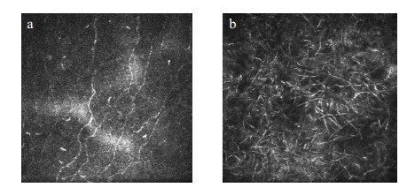
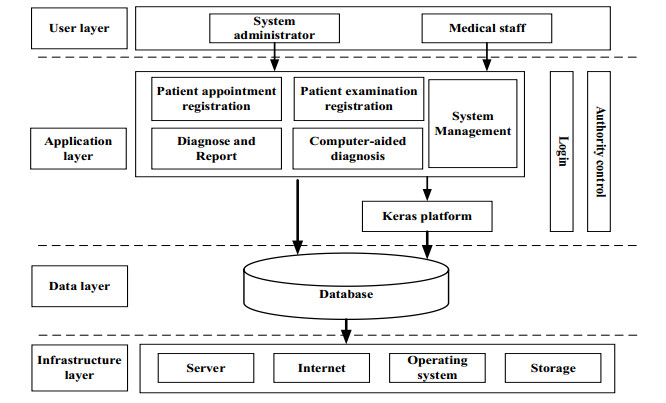
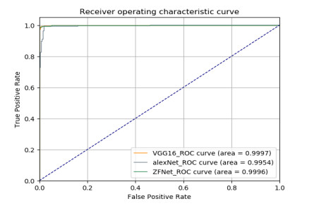
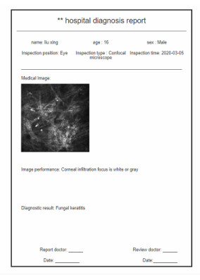
The medical image management and analysis system proposed in this paper is a medical software developed by the Browser/Server (B/S) architecture after investigating the workflow of the relevant departments of the hospital, which realizes the entire process of patients from consultation to printing of reports. The computer-aided diagnosis function is added based on image management. Due to the difficulty in collecting medical image data, in the computer-aided diagnosis module, this paper only uses the common fungal keratitis collected from the hospital in the laboratory. Focused microscope images are used for experiments. First, the images were trained with three convolutional neural networks, AlexNet, ZFNet, and VGG16. These models which classify fungal keratitis were obtained and integrated was performed to obtain better classification results. Finally, the model was integrated with the system designed in this paper, which realized the automatic diagnosis of Confocal Microscopy (CM) images of fungal keratitis online and provided it to medical staff for reference. The system can improve the work efficiency of the image-related departments while reducing the workload of doctors in the department to manually read the films.
Citation: Haixia Hou, Yankun Cao, Xiaoxiao Cui, Zhi Liu, Hongji Xu, Cheng Wang, Wensheng Zhang, Yang Zhang, Yadong Fang, Yu Geng, Wei Liang, Tie Cai, Hong Lai. Medical image management and analysis system based on web for fungal keratitis images[J]. Mathematical Biosciences and Engineering, 2021, 18(4): 3667-3679. doi: 10.3934/mbe.2021183
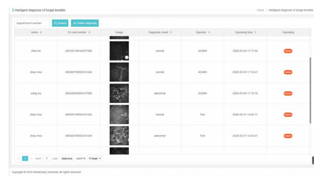
The medical image management and analysis system proposed in this paper is a medical software developed by the Browser/Server (B/S) architecture after investigating the workflow of the relevant departments of the hospital, which realizes the entire process of patients from consultation to printing of reports. The computer-aided diagnosis function is added based on image management. Due to the difficulty in collecting medical image data, in the computer-aided diagnosis module, this paper only uses the common fungal keratitis collected from the hospital in the laboratory. Focused microscope images are used for experiments. First, the images were trained with three convolutional neural networks, AlexNet, ZFNet, and VGG16. These models which classify fungal keratitis were obtained and integrated was performed to obtain better classification results. Finally, the model was integrated with the system designed in this paper, which realized the automatic diagnosis of Confocal Microscopy (CM) images of fungal keratitis online and provided it to medical staff for reference. The system can improve the work efficiency of the image-related departments while reducing the workload of doctors in the department to manually read the films.

| [1] |
P. K. Spiegel, The first clinical X-ray made in America-100 years, Am. J. Roentgenology, 164 (1995), 241-243. doi: 10.2214/ajr.164.1.7998549

|
| [2] |
I. C. Sluimer, A. M. Schilham, M. Prokop, B. Van Ginneken, Computer analysis of computed tomography scans of the lung: a survey, IEEE Trans. Med. Imaging, 25 (2006), 385-405. doi: 10.1109/TMI.2005.862753
|
| [3] |
F. Li, S. Sone, H. Abe, H. Macmahon, S. G. Armato, K. Doi, Lung cancers missed at low-dose helical CT screening in a general population: comparison of clinical, histopathologic, and imaging findings, Radiology, 225 (2002), 673-683. doi: 10.1148/radiol.2253011375
|
| [4] |
L. Xie, W. Zhong, W. Shi, S. Sun, Spectrum of fungal keratitis in north china, Ophthalmology, 113 (2006), 1943-1948. doi: 10.1016/j.ophtha.2006.05.035
|
| [5] | W. Hairong, L. Xuyang, Y. Zonghui, Design of eye health monitoring system under color fundus image visual cup segmentation algorithm, J. Med. Imaging Health Inf., 11 (2021), 277-284. |
| [6] |
A. K. Leck, P. A. Thomas, M. Hagan, J. Kaliamurthy, E. Ackuaku, M. John, et al., Aetiology of suppurative corneal ulcers in ghana and south india, and epidemiology of fungal keratitis, Br. J. Ophthalmology, 86 (2002), 1211-1215. doi: 10.1136/bjo.86.11.1211
|
| [7] |
C. A. Gonzales, M. Srinivasan, J. P. Whitcher, G. Smolin, Incidence of corneal ulceration in madurai district, south india, Ophthalmic Epidemiol., 3 (1996), 159-166. doi: 10.3109/09286589609080122
|
| [8] | X. Wu, Q. Qiu, Z. Liu, Y. Zhao, B. Zhang, Y. Zhang, Hyphae detection in fungal keratitis images with adaptive robust binary pattern, IEEE Access, 1 (2018). |
| [9] |
R. K. Mustonen, M. B. Mcdonald, S. Srivannaboon, A. L. Tan, M. W. Doubrava, C. K. Kim, Normal human corneal cell populations evaluated by in vivo scanning slit confocal microscopy, Cornea, 17 (1998), 485-492. doi: 10.1097/00003226-199809000-00005
|
| [10] |
H. Ran, C. Jiaxing, L. Yu, S. Lin, F. Chao, I. Ostfeld, Classification of deep convolutional neural network in thyroid ultrasound images, J. Med. Imaging Health Inf., 10 (2020), 1943-1948. doi: 10.1166/jmihi.2020.3099
|
| [11] |
F. Yan, Z. TaiSheng, S. Tianrong, Classification method of EEG base on evolutionary algorithm and RF for detection of epilepsy, J. Med. Imaging Health Inf., 10 (2020), 979-983. doi: 10.1166/jmihi.2020.3050
|
| [12] | A. Krizhevsky, I. Sutskever, G. Hinton, ImageNet classification with deep convolutional neural networks, Adv. Neural Informat. Process. Syst., 25 (2012). |
| [13] | M. Zeiler, R. Fergus, Visualizing and understanding convolutional networks, in European Conference on Computer Vision (ECCV), 2014. |
| [14] | K. Simonyan, A. Zisserman, Very deep convolutional networks for large-scale image recognition, preprint, arXiv: 1409.1556. |
| [15] | L.Yunhua, L. I. Quan, Research and application of network public opinion management system based on mvc model, Mod. Electron. Tech., 40 (2017), 31-33. |
| [16] | L. Ying, Y. Ming, W. Rui, W. Shuang, C. Qing, Exploration and application of wind parameter query service system based on springboot framework, Software Guide, 18 (2019), 110-113. |
| [17] | W. Dan, S. Xiaoyu, Y. Lubin, G. Shengyan, C. Center, Statistical analysis system for software based on springboot, Software Eng., 20 (2019), 40-42. |
| [18] | K. Mershad, MQL: mixed query language for querying mySQL and HBase databases, in International Conference on Innovative Trends in Computer Engineering (ITCE), IEEE, (2019), 124-129. |
Figures(9) / Tables(9)

Haixia Hou, Yankun Cao, Xiaoxiao Cui, Zhi Liu, Hongji Xu, Cheng Wang, Wensheng Zhang, Yang Zhang, Yadong Fang, Yu Geng, Wei Liang, Tie Cai, Hong Lai. Medical image management and analysis system based on web for fungal keratitis images[J]. Mathematical Biosciences and Engineering, 2021, 18(4): 3667-3679. doi: 10.3934/mbe.2021183


 DownLoad: