Dual-phase lag model of heat transfer between blood vessel and biological tissue

Ewa Majchrzak; Mikołaj Stryczyński; Ewa Majchrzak; Mikołaj Stryczyński

doi:10.3934/mbe.2021081

Mathematical Biosciences and Engineering

2021, Volume 18, Issue 2: 1573-1589. doi: 10.3934/mbe.2021081

Previous Article Next Article

Research article Special Issues

Dual-phase lag model of heat transfer between blood vessel and biological tissue

Ewa Majchrzak ^,,
Mikołaj Stryczyński

Department of Computational Mechanics and Engineering, Silesian University of Technology Gliwice, Poland

Received: 15 December 2020 Accepted: 18 January 2021 Published: 01 February 2021

A single blood vessel surrounded by the biological tissue with a tumor is considered. The influence of the heating technique (e.g. ultrasound, microwave, etc.) is described by setting a fixed temperature for the tumor which is higher than the blood and tissue temperature. The temperature distribution for the blood sub-domain is described by the energy equation written in the dual-phase lag convention, the temperature distribution in the biological tissue with a tumor is described also by the dual-phase lag equation. The boundary condition on the contact surface between blood vessel and biological tissue and the Neumann condition are also formulated using the extended Fourier law. So far in the literature, the temperature distribution in a blood vessel has been described by the classical energy equation. It is not clear whether the Fourier's law applies to highly heated tissues in which a significant thermal blood vessel is distinguished, therefore, taking into account the heterogeneous inner structure of the blood, the dual-phase lag equation is proposed for this sub-domain. The problem is solved by means of the implicit scheme of the finite difference method. The computations were performed for various values of delay times, which were taken from the available literature, and the influence of these values on the obtained temperature distributions was discussed.
- bioheat transfer,
- thermal interaction between blood vessel and tissue,
- dual-phase lag model,
- finite difference method
Citation: Ewa Majchrzak, Mikołaj Stryczyński. Dual-phase lag model of heat transfer between blood vessel and biological tissue[J]. Mathematical Biosciences and Engineering, 2021, 18(2): 1573-1589. doi: 10.3934/mbe.2021081

Related Papers:

Abstract

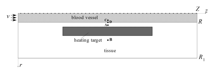
A single blood vessel surrounded by the biological tissue with a tumor is considered. The influence of the heating technique (e.g. ultrasound, microwave, etc.) is described by setting a fixed temperature for the tumor which is higher than the blood and tissue temperature. The temperature distribution for the blood sub-domain is described by the energy equation written in the dual-phase lag convention, the temperature distribution in the biological tissue with a tumor is described also by the dual-phase lag equation. The boundary condition on the contact surface between blood vessel and biological tissue and the Neumann condition are also formulated using the extended Fourier law. So far in the literature, the temperature distribution in a blood vessel has been described by the classical energy equation. It is not clear whether the Fourier's law applies to highly heated tissues in which a significant thermal blood vessel is distinguished, therefore, taking into account the heterogeneous inner structure of the blood, the dual-phase lag equation is proposed for this sub-domain. The problem is solved by means of the implicit scheme of the finite difference method. The computations were performed for various values of delay times, which were taken from the available literature, and the influence of these values on the obtained temperature distributions was discussed.

References

[1]	H. H. Pennes, Analysis of tissue and arterial blood temperatures in the resting human forearm, J. Appl. Physiol., 1 (1948), 3–23. doi: 10.1152/jappl.1948.1.1.3
[2]	M. C. Cattaneo, A form of heat conduction equation which eliminates the paradox of instantaneous propagation, C.R. Acad. Sci. I - Math., 247 (1958), 431–433.
[3]	P. Vernotte, Les paradoxes de la theorie continue de l'equation de la chaleur, Comp. Rend., 246 (1948), 3154–3155.
[4]	D. Y. Tzou, A unified field approach for heat conduction from macro- to micro- scales, J. Heat Transfer, 117 (1995), 8–16. doi: 10.1115/1.2822329
[5]	J. Crezee, J. W. Lagendijk, Temperature uniformity during hyperthermia: the impact of large vessels, Phys. Med. Biol., 37 (1992), 1321–1337. doi: 10.1088/0031-9155/37/6/009
[6]	T. C. Shih, H. L. Liu, T. L. Horng, Cooling effect of thermally significant blood vessels in perfused tumor tissue during thermal therapy, Int. Commun. Heat Mass Transfer, 33 (2006), 135–141. doi: 10.1016/j.icheatmasstransfer.2005.08.003
[7]	T. C. Shih, T. L. Horng, H. W. Huang, K. C. Ju, T. C. Huang, P. Y. Chen, et al., Numerical analysis of coupled effects of pulsatile blood flow and thermal relaxation time during thermal therapy, Int. J. Heat Mass Transfer, 55 (2012), 3763–3773. doi: 10.1016/j.ijheatmasstransfer.2012.02.069
[8]	K. Khanafer, J. L. Bull, I. Pop, R. Berguer, Influence of pulsatile blood flow and heating scheme on the temperature distribution during hyperthermia treatment, Int. J. Heat Mass Transfer, 50 (2007), 4883–4890. doi: 10.1016/j.ijheatmasstransfer.2007.01.062
[9]	M. Jamshidi, J. Ghazanfarian, Blood flow effects in thermal treatment of three-dimensional non-Fourier multilayered skin structure, Heat Transfer Eng., 2020 (2020), 1–18.
[10]	J. R. Ho, C. P. Kuo, W. S. Jiaung, Study of heat transfer in multilayered structure within the framework of dual-phase-lag heat conduction model using lattice Boltzmann method, Int. J. Heat Mass Transfer, 46 (2003), 55–69. doi: 10.1016/S0017-9310(02)00260-0
[11]	E. Majchrzak, G. Kałuża, Analysis of thermal processes occurring in the heated multilayered metal films using the dual-phase lag model, Arch. Mech., 69 (2017), 275–287.
[12]	E. Majchrzak, B. Mochnacki, Dual-phase lag model of thermal processes in a multi-layered microdomain subjected to a strong laser pulse using the implicit scheme of FDM, Int. J. Therm. Sci., 13 (2018), 240–251.
[13]	G. Hauke, An Introduction to Fluid Mechanics and Transport Phenomena, Springer, New York, 2008.
[14]	M. Ciesielski, B. Mochnacki, E. Majchrzak, Integro-differential form of the first-order dual phase lag heat transfer equation and its numerical solution using the Control Volume Method, Arch. Mech., 72 (2020), 415–444.
[15]	J. C. Chato, Heat transfer to blood vessels, J. Biomech. Eng., 102 (1980), 110–118. doi: 10.1115/1.3138205
[16]	D. A. Torvi, J. D. Dale, A finite element model of skin subjected to a flash fire, J. Biomech. Eng., 116 (1994), 250–255. doi: 10.1115/1.2895727
[17]	W. Kaminski, Hyperbolic heat conduction equation for materials with a nonhomogeneous inner structure, J. Heat Transfer, 112 (1990), 555–560. doi: 10.1115/1.2910422
[18]	Y. Zhang, Generalized dual-phase lag bioheat equations based on nonequilibrium heat transfer in living biological tissues, Int. J. Heat Mass Transfer, 52 (2009), 4829–4834. doi: 10.1016/j.ijheatmasstransfer.2009.06.007
[19]	B. Mochnacki, E. Majchrzak, Numerical model of thermal interactions between cylindrical cryoprobe and biological tissue using the dual-phase lag equation, Int. J. Heat Mass Transfer, 108 (2017), 1–10. doi: 10.1016/j.ijheatmasstransfer.2016.11.103

Reader Comments

Your name:*

Email:*
© 2021 the Author(s), licensee AIMS Press. This is an open access article distributed under the terms of the Creative Commons Attribution License (http://creativecommons.org/licenses/by/4.0)