Dynamic analysis and control of online information dissemination model considering information beneficiaries

Xuechao Zhang; Yuhan Hu; Shichang Lu; Haomiao Guo; Xiaoyan Wei; Jun li; Xuechao Zhang; Yuhan Hu; Shichang Lu; Haomiao Guo; Xiaoyan Wei; Jun li

doi:10.3934/math.2025229

AIMS Mathematics

2025, Volume 10, Issue 3: 4992-5020. doi: 10.3934/math.2025229

Previous Article Next Article

Research article

Dynamic analysis and control of online information dissemination model considering information beneficiaries

1.
School of Business Administration, Liaoning Technical University, Huludao, Liaoning, China
2.
School of Science, University of Science and Technology Liaoning, Anshan, Liaoning, China
3.
School of Economics and Law, University of Science and Technology Liaoning, Anshan, Liaoning, China

Received: 19 December 2024 Revised: 20 February 2025 Accepted: 27 February 2025 Published: 06 March 2025
MSC : 34D20, 49J15, 37D35

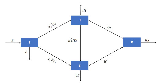
With the rapid rise and widespread adoption of social media, theoretical research on the dynamics of online information dissemination has become increasingly important. Therefore, we developed a new model of information diffusion that took into account the influence of information recipients on the diffusion of information. First, initially, the basic reproduction number of the model was calculated. Then, we analyzed the existence and stability of the equilibrium point. Next, based on the principle of Pontryagin's maximum principle, a control strategy was derived to effectively enhance the propagation of information. Numerical simulations verified the results of theoretical analysis. The results showed that increasing the proportion of propagators and the probability of beneficiaries transitioning into propagators significantly accelerated the speed and extent of information diffusion.
- information spreading,
- information beneficiaries,
- basic reproduction number,
- differential equation,
- stability analysis
Citation: Xuechao Zhang, Yuhan Hu, Shichang Lu, Haomiao Guo, Xiaoyan Wei, Jun li. Dynamic analysis and control of online information dissemination model considering information beneficiaries[J]. AIMS Mathematics, 2025, 10(3): 4992-5020. doi: 10.3934/math.2025229

Related Papers:

Abstract

With the rapid rise and widespread adoption of social media, theoretical research on the dynamics of online information dissemination has become increasingly important. Therefore, we developed a new model of information diffusion that took into account the influence of information recipients on the diffusion of information. First, initially, the basic reproduction number of the model was calculated. Then, we analyzed the existence and stability of the equilibrium point. Next, based on the principle of Pontryagin's maximum principle, a control strategy was derived to effectively enhance the propagation of information. Numerical simulations verified the results of theoretical analysis. The results showed that increasing the proportion of propagators and the probability of beneficiaries transitioning into propagators significantly accelerated the speed and extent of information diffusion.

References

[1]	M. Castells, Toward a sociology of the network society, Contemp. Sociol., 29 (2000), 693–699. https://doi.org/10.2307/2655234 doi: 10.2307/2655234
[2]	J. H. Kietzmann, K. Hermkens, I. P. Mccarthy, B. S. Silvestre, Social media? Get serious! Understanding the functional building blocks of social media, Bus. Horizons, 54 (2011), 241–251. http://dx.doi.org/10.1016/j.bushor.2011.01.005 doi: 10.1016/j.bushor.2011.01.005
[3]	S. Funk, E. Gilad, C. Watkins, V. A. Jansen, The spread of awareness and its impact on epidemic outbreaks, P. Natl. Acad. Sci., 106 (2009), 6872–6877. http://dx.doi.org/10.1073/pnas.0810762106 doi: 10.1073/pnas.0810762106
[4]	S. Lewandowsky, U. K. H. Ecker, J. Cook, Beyond misinformation: Understanding and coping with the "post-truth" era, J. Appl. Res. Mem. Cogn., 6 (2017), 353–369. http://dx.doi.org/10.1016/j.jarmac.2017.07.008 doi: 10.1016/j.jarmac.2017.07.008
[5]	A. E. Marwick, R. Lewis, Media manipulation and disinformation online, J. Amer. Math. Soc., 2017.
[6]	T. Preis, H. S. Moat, H. E. Stanley, Quantifying trading behavior in financial markets using google trends, Sci. Rep., 3 (2013), 1684–1684. http://dx.doi.org/10.1090/S0894-0347-1992-1124979-1 doi: 10.1090/S0894-0347-1992-1124979-1
[7]	H. S. Moat, C. Curme, A. Avakian, D. Y. Kenett, H. E. Stanley, T. Preis, Quantifying wikipedia usage patterns before stock market moves, Sci. Rep., 3 (2013), 2045–2322. http://dx.doi.org/10.1038/srep01801 doi: 10.1038/srep01801
[8]	Q. L. Yan, S. Y. Tang, S. Gabriele, J. H. Wu, Media coverage and hospital notifications: Correlation analysis and optimal media impact duration to manage a pandemic, J. Theor. Biol., 390 (2016), 1–13. http://dx.doi.org/10.1090/S0894-0347-1992-1124979-1 doi: 10.1090/S0894-0347-1992-1124979-1
[9]	R. Ross, H. P. Hudson, An application of the theory of probabilities to the study of a priori pathometry, Part Ⅲ, Proc. R. Soc. Lond. A, 89 (1917), 225–240. http://dx.doi.org/10.1098/rspa.1917.0015 doi: 10.1098/rspa.1917.0015
[10]	D. J. Daley, D. G. Kendall, Epidemics and rumours, Nature, 204 (1964), 1118–1118. https://doi.org/10.1038/2041118a0 doi: 10.1038/2041118a0
[11]	D. J. Daley, D. G. Kendall, Stochastic rumours, Ima J. Appl. Math., 1 (1965), 42–55. https://doi.org/10.1093/imamat/1.1.42 doi: 10.1093/imamat/1.1.42
[12]	R. Schweizer, Mathematical models and applications: With emphasis on the social, life, and management sciences, 2016.
[13]	S. J. Gao, Z. D. Teng, J. J. Nieto, T. Angela, Analysis of an SIR epidemic model with pulse vaccination and distributed time delay, J. Biomed. Biotechnol., 2007 (2007), 1–10. http://dx.doi.org/10.1155/2007/64870 doi: 10.1155/2007/64870
[14]	Y. Liu, S. M. Diao, Y. X. Zhu, Q. Liu, SHIR competitive information diffusion model for online social media, Physica A, 461 (2016), 543–553. http://dx.doi.org/10.1016/j.physa.2016.06.080 doi: 10.1016/j.physa.2016.06.080
[15]	Q. Liu, D. Q. Jiang, T. Hayat, B. Ahmad, Anosov flows with stable and unstable differentiable distributions, Nonlinear Anal.- Hybri., 27 (2018), 29–43. http://dx.doi.org/10.1016/j.nahs.2017.08.002 doi: 10.1016/j.nahs.2017.08.002
[16]	Q. Liu, Q. M. Chen, D. Q. Jiang, The threshold of a stochastic delayed SIR epidemic model with temporary immunity, Physica A, 450 (2016), 115–125. http://dx.doi.org/10.1016/j.physa.2015.12.056 doi: 10.1016/j.physa.2015.12.056
[17]	C. Wan, T. Li, Z. H. Guan, Y. M. Wang, X. D. Liu, Spreading dynamics of an e-commerce preferential information model on scale-free networks, Physica A, 467 (2017), 192–200. http://dx.doi.org/10.1016/j.physa.2016.09.035 doi: 10.1016/j.physa.2016.09.035
[18]	Y. M. Zhang, Y. Y. Su, W. G. Li, H. O. Liu, Rumor and authoritative information propagation model considering super spreading in complex social networks, Physica A, 506 (2018), 359–411. http://dx.doi.org/10.1016/j.physa.2018.04.082 doi: 10.1016/j.physa.2018.04.082
[19]	S. Hosseini, M. A. Abdollahi, The dynamics of an SEIRS-QV malware propagation model in heterogeneous networks, Physica A, 512 (2018), 803–817. http://dx.doi.org/10.1016/j.physa.2018.08.081 doi: 10.1016/j.physa.2018.08.081
[20]	F. Wu, B. A. Huberman, Social structure and opinion formation, Comput. Econ., 2004. https://doi.org/10.48550/arXiv.cond-mat/0407252
[21]	M. Small, C. K. Tse, D. M. Walker, Super-spreaders and the rate of transmission of the SARS virus, Physica D, 215 (2006), 146–158. http://dx.doi.org/10.1016/j.physd.2006.01.021 doi: 10.1016/j.physd.2006.01.021
[22]	L. L. Weng, A. Flammini, A. Vespignani, F. Menczer, Competition among memes in a world with limited attention, Sci. Rep., 2 (2012), 335–335. http://dx.doi.org/10.1038/srep00335 doi: 10.1038/srep00335
[23]	A. Guille, H. Hacid, C. Favre, D. A. Zighed, Information diffusion in online social networks: A Survey, SIGMOD Rec., 42 (2013), 17–28. http://dx.doi.org/10.1145/2503792.2503797 doi: 10.1145/2503792.2503797
[24]	J. B. Holthoefer, S. Meloni, B. Gonçalves, Y. Moreno, Emergence of influential spreaders in modified rumor models, J. Stat. Phys., 151 (2013), 383–393. http://dx.doi.org/10.1007/s10955-012-0595-6 doi: 10.1007/s10955-012-0595-6
[25]	K. Lerman, R. Ghosh, Information contagion: An empirical study of the spread of news on digg and twitter social networks, In: Proceedings of the International AAAI Conference on Web and Social Media, 52 (2010), 166–176. https://doi.org/10.1609/icwsm.v4i1.14021
[26]	N. Carbonara, Information and communication technology and geographical clusters: Opportunities and spread, Technovation, 25 (2005), 213–222. http://dx.doi.org/10.1016/s0166-4972(03)00095-6 doi: 10.1016/s0166-4972(03)00095-6
[27]	M. Salehi, R. Sharma, M. Marzolla, M. Magnani, P. Siyari, D. Montesi, Spreading processes in multilayer networks, IEEE T. Netw. Sci. Eng., 2 (2015), 65–83. http://dx.doi.org/10.1109/TNSE.2015.2425961 doi: 10.1109/TNSE.2015.2425961
[28]	L. P. Fu, B. Hellinga, Real-time, adaptive prediction of incident delay for advanced traffic management and information systems, J. Am. Math. Soc., 2002, 12–15. http://dx.doi.org/10.1090/S0894-0347-1992-1124979-1 doi: 10.1090/S0894-0347-1992-1124979-1
[29]	S. Y. Sun, H. Y. Liu, J. He, X. Y. Du, Web technologies and applications: Detecting event rumors on sina weibo automatically, Berlin, Heidelberg: Springer, 7808 (2013), 120–131. https://doi.org/10.1007/978-3-642-37401-2-14
[30]	S. Kang, X. L. Hou, Y. H. Hu, H. Y. Liu, Dynamical analysis and optimal control of the developed information transmission model, PLOS One, 17 (2022). https://doi.org/10.1371/journal.pone.0268326 doi: 10.1371/journal.pone.0268326
[31]	S. F. Marinósson, Lyapunov function construction for ordinary differential equations with linear programming, Dynam. Syst., 17 (2002), 137–150. https://doi.org/10.1080/0268111011011847 doi: 10.1080/0268111011011847
[32]	J. P. Lasalle, The stability of dynamical systems, SIAM, 1976.
[33]	Y. Zhang, Z. Chen, SETQR propagation model for social networks, IEEE Access, 7 (2019), 127533–127543. https://doi.org/10.1109/ACCESS.2019.2939150 doi: 10.1109/ACCESS.2019.2939150
[34]	A. Foligno, P. Kos, B. Bertini, Quantum information spreading in generalized dual-unitary circuits, Phys. Rev. Lett., 132 (2024), 250402. https://10.1103/physrevlett.132.250402 doi: 10.1103/physrevlett.132.250402
[35]	W. Q. Pan, W. J. Yan, Y. H. Hu, R. M. He, L. B. Wu, G. Rasool, Dynamic analysis and optimal control of rumor propagation model with reporting effect, Adv. Math. Phys., 2022 (2022), 1–14. https://doi.org/10.1155/2022/5503137 doi: 10.1155/2022/5503137
[36]	M. Hale, Y. Wardi, H. Jaleel, M. Egerstedt, Hamiltonian-based algo rithm for optimal control, arXiv Preprint, 2016. https://doi.org/10.48550/arXiv.1603.02747
[37]	L. Bittner, L. S. Pontryagin, V. G. Boltyanskii, R. V. Gamkrelidze, E. F. Mishchenko, The mathematical theory of optimal processes, New York: John Wiley & Sons, 43 (1962), 514–515. https://doi.org/10.1002/zamm.19630431023
[38]	K. Hattaf, A new mixed fractional derivative with applications in computational biology, Computation, 1 (2024), 7. https://doi.org/10.3390/computation12010007 doi: 10.3390/computation12010007

Reader Comments

Your name:*

Email:*
© 2025 the Author(s), licensee AIMS Press. This is an open access article distributed under the terms of the Creative Commons Attribution License (http://creativecommons.org/licenses/by/4.0)