The new soliton solution types to the Myrzakulov-Lakshmanan-XXXII-equation

Emad H. M. Zahran; Ahmet Bekir; Reda A. Ibrahim; Ratbay Myrzakulov; Emad H. M. Zahran; Ahmet Bekir; Reda A. Ibrahim; Ratbay Myrzakulov

doi:10.3934/math.2024300

AIMS Mathematics

2024, Volume 9, Issue 3: 6145-6160. doi: 10.3934/math.2024300

Previous Article Next Article

Research article

The new soliton solution types to the Myrzakulov-Lakshmanan-XXXII-equation

1.
Department of Basic Science, Benha University, Faculty of Engineering, Shubra, Egypt
2.
Neighbourhood of Akcaglan, Imarli Street, Number: 28/4, 26030, Eskisehir, Turkey
3.
Departments of Basic Science, Benha University, Faculty of Engineering, Shubra, Egypt
4.
Ratbay Myrzakulov Eurasian International Centre for Theoretical Physics, Astana, Kazakhstan

Received: 13 December 2023 Revised: 19 January 2024 Accepted: 23 January 2024 Published: 02 February 2024
MSC : 35C07, 35Q51, 83C15

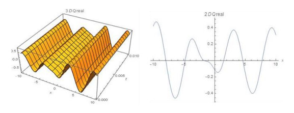
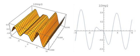
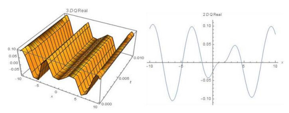
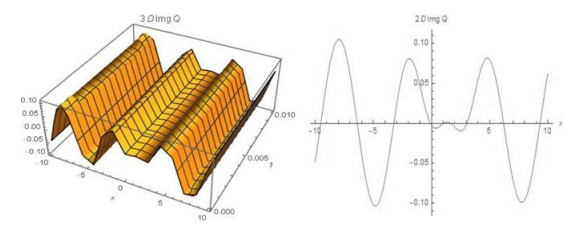
Our attention concenters on deriving diverse forms of the soliton arising from the Myrzakulov-Lakshmanan XXXII (M-XXXII) that describes the generalized Heisenberg ferromagnetic equation. This model has been solved numerically only using the N-fold Darboux Transformation method, not solved analytically before. We will derive new types of the analytical soliton solutions that will be constructed for the first time in the framework of three impressive schemas that are prepared for this target. These three techniques are the Generalized Kudryashov scheme (GKS), the (G'/G)-expansion scheme and the extended direct algebraic scheme (EDAS). Moreover, we will establish the 2D, 3D graphical simulations that clear the new dynamic properties of our achieved solutions.
Citation: Emad H. M. Zahran, Ahmet Bekir, Reda A. Ibrahim, Ratbay Myrzakulov. The new soliton solution types to the Myrzakulov-Lakshmanan-XXXII-equation[J]. AIMS Mathematics, 2024, 9(3): 6145-6160. doi: 10.3934/math.2024300

Related Papers:

Abstract

Our attention concenters on deriving diverse forms of the soliton arising from the Myrzakulov-Lakshmanan XXXII (M-XXXII) that describes the generalized Heisenberg ferromagnetic equation. This model has been solved numerically only using the N-fold Darboux Transformation method, not solved analytically before. We will derive new types of the analytical soliton solutions that will be constructed for the first time in the framework of three impressive schemas that are prepared for this target. These three techniques are the Generalized Kudryashov scheme (GKS), the (G'/G)-expansion scheme and the extended direct algebraic scheme (EDAS). Moreover, we will establish the 2D, 3D graphical simulations that clear the new dynamic properties of our achieved solutions.

References

[1]	L. Debnath, Nonlinear partial differential equations for scientists and engineers, Massachusetts: Birkhäuser Boston, 2005. https://doi.org/10.1007/b138648
[2]	J. Yu, B. Ren, P. Liu, J. Zhou, CTE solvability, nonlocal symmetry, and interaction solutions of coupled integrable dispersion-less system, Complexity, 2022 (2022), 32211447. https://doi.org/10.1155/2022/3221447
[3]	K. Takasaki, Dispersionless Toda hierarchy and two-dimensional string theory, Commun. Math. Phys., 170 (1995), 101–116. https://doi.org/10.1007/BF02099441 doi: 10.1007/BF02099441
[4]	S. Aoyama, Y. Kodama, Topological conformal field theory with a rational W potential and the dispersionless KP hierarchy, Mod. Phys. Lett. A, 9 (1994), 2481–2492. https://doi.org/10.1142/S0217732394002355 doi: 10.1142/S0217732394002355
[5]	Z. Sagidullayeva, K. Yesmakhanova, R. Myrzakulov, Z. Myrzakulova, N. Serikbayev, G. Nugmanova, et al., Integrable generalized Heisenberg ferromagnet equations in 1+1 dimensions: reductions and gauge equivalence, arXiv: 2205.02073.
[6]	R. Myrzakulov, On some sigma models with potentials and the Klein-Gordon type equations, arXiv: hep-th/9812214.
[7]	K. Yesmakhanova, G. Nugmanova, G. Shaikhova, G. Bekova, R. Myrzakulov, Coupled dispersionless and generalized Heisenberg ferromagnet equations with self-consistent sources: geometry and equivalence, Int. J. Geom. Methods M., 17 (2020), 2050104. https://doi.org/10.1142/S0219887820501042 doi: 10.1142/S0219887820501042
[8]	M. Latha, C. Christal Vasanthi, An integrable model of (2+1)-dimensional Heisenberg ferromagnetic spin chain and soliton excitations, Phys. Scr., 89 (2014), 065204. https://doi.org/10.1088/0031-8949/89/6/065204
[9]	H. Triki, A. Wazwaz, New solitons and periodic wave solutions for the (2+1) dimensional Heisenberg ferromagnetic spin chain equation, J. Electromagnet. Wave., 30 (2016), 788–794. https://doi.org/10.1080/09205071.2016.1153986 doi: 10.1080/09205071.2016.1153986
[10]	M. Inc, A. Aliyu, A. Yusuf, D. Baleanu, Optical solitons and modulation instability analysis of an integrable model of (2+1)-Dimensional Heisenberg ferromagnetic spin chain equation, Micro Nanostructures, 112 (2017), 628–638. https://doi.org/10.1016/j.spmi.2017.10.018 doi: 10.1016/j.spmi.2017.10.018
[11]	S. Rayhanul Islam, M. Bashar, N. Muhammad, Immeasurable soliton solutions and enhanced (G'/G)-expansion method, Physics Open, 9 (2021), 100086. https://doi.org/10.1016/j.physo.2021.100086 doi: 10.1016/j.physo.2021.100086
[12]	B. Deng, H. Hao, Breathers, rogue waves and semi-rational solutions for a generalized Heisenberg ferromagnetic equation, Appl. Math. Lett., 140 (2023), 108550. https://doi.org/10.1016/j.aml.2022.108550
[13]	M. Daniel, L. Kavitha, R. Amuda, Soliton spin excitations in an anisotropic Heisenberg ferromagnet with octupole-dipole interaction, Phys. Rev. B, 59 (1999), 13774. https://doi.org/10.1103/PhysRevB.59.13774 doi: 10.1103/PhysRevB.59.13774
[14]	H. Triki, A. Wazwaz, New solitons and periodic wave solutions for the (2+1) dimensional Heisenberg ferromagnetic spin chain equation, J. Electromagnet. Wave., 30 (2016), 788–794. https://doi.org/10.1080/09205071.2016.1153986 doi: 10.1080/09205071.2016.1153986
[15]	M. Bashar, S. Rayhanul Islam, D. Kumar, Construction of traveling wave solutions of the (2+1)-dimensional Heisenberg ferromagnetic spin chain equation, Partial Differential Equations in Applied Mathematics, 4 (2021), 100040. https://doi.org/10.1016/j.padiff.2021.100040 doi: 10.1016/j.padiff.2021.100040
[16]	M. Bashar, S. Rayhanul Islam, Exact solutions to the (2+1)-Dimensional Heisenberg ferromagnetic spin chain equation by using modified simple equation and improve F-expansion methods, Physics Open, 5 (2020), 100027. https://doi.org/10.1016/j.physo.2020.100027
[17]	C. Christal Vasanthi, M. Latha, Heisenberg ferromagnetic spin chain with bilinear and biquadratic interactions in (2+1)-dimensions, Commun. Nonlinear Sci., 28 (2015), 109–122. https://doi.org/10.1016/j.cnsns.2015.04.012 doi: 10.1016/j.cnsns.2015.04.012
[18]	E. Zahran, A. Bekir, New unexpected variety of solitons arising from spatio-temporal dispersion (1+1) dimensional Ito-equation, Mod. Phys. Lett. B, 38 (2024), 2350258. https://doi.org/10.1142/S0217984923502585 doi: 10.1142/S0217984923502585
[19]	E. Zahran, A. Bekir, Optical soliton solutions to the perturbed Biswas-Milovic equation with Kudryashov's law of refractive index, Opt. Quant. Electron., 55 (2023), 1211. https://doi.org/10.1007/s11082-023-05453-w doi: 10.1007/s11082-023-05453-w
[20]	S. Kumar, R. Jiwari, R. Mittal, J. Awrejcewicz, Dark and bright soliton solutions and computational modeling of nonlinear regularized long wave model, Nonlinear Dyn., 104 (2021), 661–682. https://doi.org/10.1007/s11071-021-06291-9 doi: 10.1007/s11071-021-06291-9
[21]	E. Zahran, A. Bekir, New unexpected soliton solutions to the generalized (2+1) Schrödinger equation with its four mixing waves, Int. J. Mod. Phys. B, 36 (2022), 2250166. https://doi.org/10.1142/S0217979222501661 doi: 10.1142/S0217979222501661
[22]	M. Younis, T. Sulaiman, M. Bilal, S. Ur Rehman, U. Younas, Modulation instability analysis optical and other solutions to the modified nonlinear Schrödinger equation, Commun. Theor. Phys., 72 (2020), 065001. https://doi.org/10.1088/1572-9494/ab7ec8 doi: 10.1088/1572-9494/ab7ec8
[23]	E. Zahran, A. Bekir, R. Ibrahim, New optical soliton solutions of the popularized anti-cubic nonlinear Schrödinger equation versus its numerical treatment, Opt. Quant. Electron., 55 (2023), 377. https://doi.org/10.1007/s11082-023-04624-z doi: 10.1007/s11082-023-04624-z
[24]	E. Zahran, A. Bekir, M. Shehata, New diverse variety analytical optical soliton solutions for two various models that are emerged from the perturbed nonlinear Schrödinger equation, Opt. Quant. Electron., 55 (2023), 190. https://doi.org/10.1007/s11082-022-04423-y doi: 10.1007/s11082-022-04423-y
[25]	M. Ali Akbar, A. Wazwaz, F. Mahmud, D. Baleanu, R. Roy, H. Barman, et al., Dynamical behavior of solitons of the perturbed nonlinear Schrödinger equation and microtubules through the generalized Kudryashov scheme, Results Phys., 43 (2022), 106079. https://doi.org/10.1016/j.rinp.2022.106079
[26]	L. Ouahid, S. Owyed, M. Abdou, N. Alshehri, S. Elagan, New optical soliton solutions via generalized Kudryashov's scheme for Ginzburg-Landau equation in fractal order, Alex. Eng. J., 60 (2021), 5495–5510. https://doi.org/10.1016/j.aej.2021.04.030 doi: 10.1016/j.aej.2021.04.030
[27]	G. Genc, M. Ekici, A. Biswas, M. Belic, Cubic-quartic optical solitons with Kudryashov's law of refractive index by F-expansions schemes, Results Phys., 18 (2020), 103273. https://doi.org/10.1016/j.rinp.2020.103273 doi: 10.1016/j.rinp.2020.103273
[28]	D. Kumar, A. Seadawy, A. Joardar, Modified Kudryashov method via new exact solutions for some conformable fractional differential equations arising in mathematical biology, Chinese J. Phys., 56 (2018), 75–85. https://doi.org/10.1016/j.cjph.2017.11.020 doi: 10.1016/j.cjph.2017.11.020
[29]	C. Gomez S, H. Roshid, M. Inc, L. Akinyemi, H. Rezazadeh, On soliton solutions for perturbed Fokas-Lenells equation, Opt. Quant. Electron., 54 (2022), 370. https://doi.org/10.1007/s11082-022-03796-4 doi: 10.1007/s11082-022-03796-4
[30]	E. Zahran, A. Bekir, New variety diverse solitary wave solutions to the DNA Peyrard-Bishop model, Mod. Phys. Lett. B, 37 (2023), 2350027. https://doi.org/10.1142/S0217984923500276 doi: 10.1142/S0217984923500276
[31]	E. Zahran, A. Bekir, New solitary solutions to the nonlinear Schrödinger equation under the few-cycle pulse propagation property, Opt. Quant. Electron., 55 (2023), 696. https://doi.org/10.1007/s11082-023-04916-4 doi: 10.1007/s11082-023-04916-4
[32]	E. Zahran, A. Bekir, New diverse soliton solutions for the coupled Konno-Oono equations, Opt. Quant. Electron., 55 (2023), 112. https://doi.org/10.1007/s11082-022-04376-2 doi: 10.1007/s11082-022-04376-2
[33]	E. Zahran, H. Ahmad, T. Saeed, T. Botmart, New diverse variety for the exact solutions to Keller-Segel-Fisher system, Results Phys., 35 (2022), 105320. https://doi.org/10.1016/j.rinp.2022.105320 doi: 10.1016/j.rinp.2022.105320
[34]	A. Hyder, M. Barakat, General improved Kudryashov method for exact solutions of nonlinear evolution equations in mathematical physics, Phys. Scr., 95 (2020), 045212. https://doi.org/10.1088/1402-4896/ab6526 doi: 10.1088/1402-4896/ab6526

Reader Comments

Your name:*

Email:*
© 2024 the Author(s), licensee AIMS Press. This is an open access article distributed under the terms of the Creative Commons Attribution License (http://creativecommons.org/licenses/by/4.0)