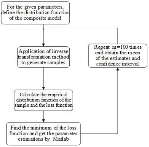
Threshold selection is challenging when analyzing tail data with a generalized Pareto distribution. Data below the threshold was not used in the model, resulting in incomplete characterization of the whole data. This paper applied the Gamma distribution, Weibull distribution, and lognormal distribution to fit the central data separately, and a generalized Pareto distribution (GPD) was used to analyze the tail data. In such composite models, the thresholds are estimated directly as parameters. We proposed an empirical distribution function-based parameter estimation method. The absolute value of the difference between the empirical distribution function and the composite distribution function was used as a loss function to obtain an estimate of the parameter. This parameter estimation method is suitable for complex multiparameter distributions. The estimation method based on the empirical distribution function was verified to be feasible through simulation studies. The composite model and the estimation method based on the empirical distribution function were applied to study the earthquake magnitude data to provide a reference for earthquake hazard analysis.
Citation: Yanfang Zhang, Fuchang Wang, Yibin Zhao. Statistical characteristics of earthquake magnitude based on the composite model[J]. AIMS Mathematics, 2024, 9(1): 607-624. doi: 10.3934/math.2024032
Threshold selection is challenging when analyzing tail data with a generalized Pareto distribution. Data below the threshold was not used in the model, resulting in incomplete characterization of the whole data. This paper applied the Gamma distribution, Weibull distribution, and lognormal distribution to fit the central data separately, and a generalized Pareto distribution (GPD) was used to analyze the tail data. In such composite models, the thresholds are estimated directly as parameters. We proposed an empirical distribution function-based parameter estimation method. The absolute value of the difference between the empirical distribution function and the composite distribution function was used as a loss function to obtain an estimate of the parameter. This parameter estimation method is suitable for complex multiparameter distributions. The estimation method based on the empirical distribution function was verified to be feasible through simulation studies. The composite model and the estimation method based on the empirical distribution function were applied to study the earthquake magnitude data to provide a reference for earthquake hazard analysis.

| [1] | E. Castillo, Extreme value theory in engineering, 1 Eds., New York: Academic Press, 1988. https://doi.org/10.2307/1269867 |
| [2] |
V. F. Pisarenko, A. Sornette, D. Sornette, Characterization of the tail of the distribution of earthquake magnitudes by combining the GEV and GPD descriptions of extreme value theory, Pure Appl. Geophys., 171 (2014), 1599–1624. https://doi.org/10.1007/s00024-014-0882-z doi: 10.1007/s00024-014-0882-z

|
| [3] | S. Coles, An introduction to statistical modeling of extreme values, 1 Eds., Springer Series in Statistics, London: Springer-Verlag, 2001. Available from: https://www.doc88.com/p-9089129087291.html. |
| [4] |
C. Scarrott, A. Macdonald, A review of extreme value threshold estimation and uncertainty quantification authors, Revstat-Stat. J., 10 (2012), 33–60. https://doi.org/10.1111/j.1467-842X.2012.00658.x doi: 10.1111/j.1467-842X.2012.00658.x
|
| [5] | P. Embrechts, C. Klüppelberg, T. Mikosch, Modelling extremal events for insurance and finance, New York: Springer, 1997. https://doi.org/10.1007/978-3-642-33483-2 |
| [6] |
W. Dumouchel, G. Duncan, Using sample survey weights in multiple regression analyses of stratified samples, J. Am. Stat. Assoc., 78 (1983), 535–54. https://doi.org/10.1080/01621459.1983.10478006 doi: 10.1080/01621459.1983.10478006
|
| [7] |
A. Frigessi, O. Haug, H. Rue, A dynamic mixture model for unsupervised tail estimation without threshold selection, Extremes, 5 (2002), 219–235. https://doi.org/10.1023/A:1024072610684 doi: 10.1023/A:1024072610684
|
| [8] |
B. D. M. Mendes, H. F. Lopes, Data driven estimates for mixtures, Comput. Stat. Data An., 47 (2004), 583–598. https://doi.org/10.1016/j.csda.2003.12.006 doi: 10.1016/j.csda.2003.12.006
|
| [9] |
J. Carreau, Y. Bengio, A hybrid Pareto model for asymmetric fat-tailed data: the univariate case, Extremes, 12 (2009), 53–76. https://doi.org/10.1007/s10687-008-0068-0 doi: 10.1007/s10687-008-0068-0
|
| [10] |
C. N. Behrens, H. F. Lopes, D. Gamerman, Bayesian analysis of extreme events with threshold estimation, Stat. Model. Int. J., 4 (2003), 227–244. https://doi.org/10.1191/1471082X04st075oa doi: 10.1191/1471082X04st075oa
|
| [11] |
S. Nadarajah, S. A. A. Bakar, New composite models for the Danish fire insurance data, Scand. Actuar. J., 2014 (2014), 180–187. https://doi.org/10.1080/03461238.2012.695748 doi: 10.1080/03461238.2012.695748
|
| [12] |
E. C. Ojeda, On the composite Weibull-Burr model to describe claim data, Communications in Statistics: Case Studies, Data Anal. Appl., 1 (2015), 59–69. https://doi.org/10.1080/23737484.2015.1066661 doi: 10.1080/23737484.2015.1066661
|
| [13] |
E. C. Ojeda, The distribution of all French communes: A composite parametric approach, Physica A, 450 (2016), 385–394. https://doi.org/10.1016/j.physa.2016.01.018 doi: 10.1016/j.physa.2016.01.018
|
| [14] |
S. Wang, W. Chen, M. Chen, Y. W. Zhou, Maximum likelihood estimation of the parameters of the inverse Gaussian distribution using maximum rank set sampling with unequal samples, Math. Popul. Stud., 30 (2023), 1–21. https://doi.org/10.1080/08898480.2021.1996822 doi: 10.1080/08898480.2021.1996822
|
| [15] |
J. Carreau, Y. Bengio, A hybrid Pareto mixture for conditional asymmetric fat-tailed distributions, IEEE T. Neur. Networ., 20 (2009), 1087–1101. https://doi.org/10.1109/TNN.2009.2016339 doi: 10.1109/TNN.2009.2016339
|
| [16] |
J. Carreau, P. Naveau, E. Sauquet, A statistical rainfall-runoff mixture model with heavy-tailed components, Water Resour. Res., 45 (2009). https://doi.org/10.1029/2009wr007880 doi: 10.1029/2009wr007880
|
| [17] |
A. Tancredi, C. Anderson, A. O'Hagan, Accounting for threshold uncertainty in extreme value estimation, Extremes, 9 (2006), 87–106. https://doi.org/10.1007/s10687-006-0009-8 doi: 10.1007/s10687-006-0009-8
|
| [18] |
Y. X. Li, N. Tang, X. Jiang, Bayesian approaches for analyzing earthquake catastrophic risk, Insur. Math. Econ., 68 (2016), 110–119. https://doi.org/10.1016/j.insmatheco.2016.02.004 doi: 10.1016/j.insmatheco.2016.02.004
|
| [19] |
D. J. Dupuis, Exceedances over high thresholds: A guide to threshold selection, Extremes, 1 (1999), 251–261. https://doi.org/10.1023/A:1009914915709 doi: 10.1023/A:1009914915709
|
| [20] |
Y. Cai, D. Reeve, J. Stander, Automated threshold selection methods for extreme wave analysis, Coast. Eng., 56 (2009), 1013–1021. https://doi.org/10.1016/j.coastaleng.2009.06.003 doi: 10.1016/j.coastaleng.2009.06.003
|
| [21] | C. Forbes, M. Evans, N. Hastings, B. Peacock, Statistical distributions, 4 Eds., New Jersey: John Wiley & Sons, Inc., Hoboken, 2011. https://doi.org/10.1177/14614448100120051102 |
| [22] |
J. P. Iii, Statistical inference using extreme order statistics, Ann. Stat., 3 (1975), 119–131. https://doi.org/10.1214/aos/1176343003 doi: 10.1214/aos/1176343003
|
| [23] |
A. A. Balkema, L. D. Haan, Residual life time at great age, Ann. Probab., 2 (1974), 792–804. https://doi.org/10.1214/aop/1176996548 doi: 10.1214/aop/1176996548
|
| [24] | M. R. Leadbetter, G. Lindgren, H. Rootzén, Extremes and related properties of random sequences and processes, New York: Springer Science Business Media, LLC Springer Verlag, 1984. |
| [25] |
V. F. P. Sornette, Characterization of the frequency of extreme earthquake events by the generalized Pareto distribution, Pure Appl. Geophys., 160 (2003), 2343–2364. https://doi.org/10.1007/s00024-003-2397-x doi: 10.1007/s00024-003-2397-x
|
| [26] |
S. M. A. Mohd, M. Nurulkamal, I. Kamarulzaman, A robust semi-parametric approach for measuring income inequality in Malaysia, Physica A, 2018. https://doi.org/10.1016/j.physa.2018.08.029 doi: 10.1016/j.physa.2018.08.029
|


Figures(10) / Tables(13)

Yanfang Zhang, Fuchang Wang, Yibin Zhao. Statistical characteristics of earthquake magnitude based on the composite model[J]. AIMS Mathematics, 2024, 9(1): 607-624. doi: 10.3934/math.2024032


 DownLoad: