The boundedness character, persistent nature, and asymptotic conduct of non-negative outcomes of the system of three dimensional exponential form of difference equations were studied in this research:
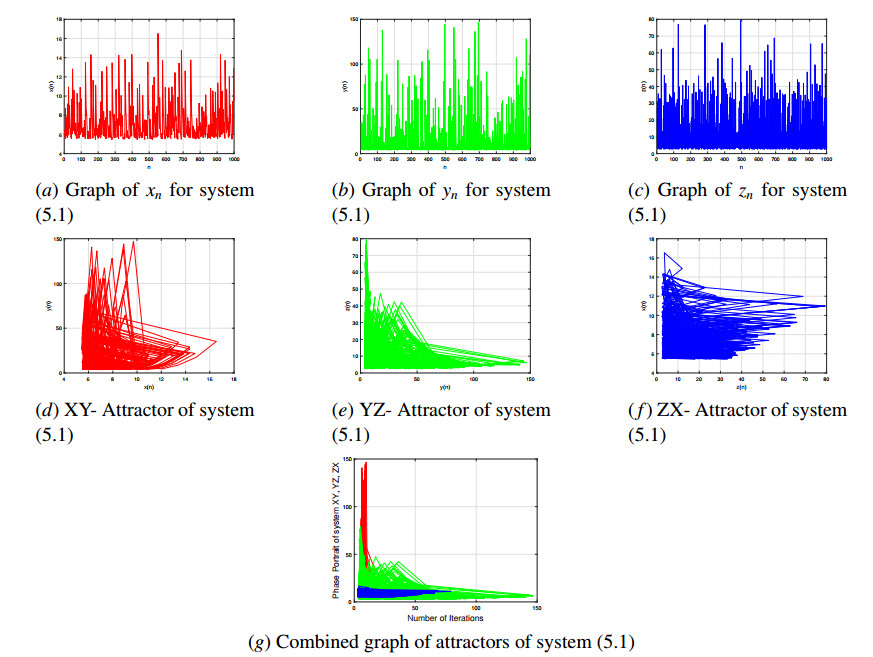
$ \begin{eqnarray*} x_{n+1} & = &ax_{n}+by_{n-1}e^{-x_{n}}, \\ \text{ }y_{n+1} & = &cy_{n}+dz_{n-1}e^{-y_{n}},\ \\ z_{n+1} & = &ez_{n}+fx_{n-1}e^{-z_{n}}, \end{eqnarray*} $
where $ a, \ b, \ c $, $ d, \ e $ and $ f $ are non-negative real values, and the initial values $ x_{-1}, \ x_{0}, \ y_{-1}, \ y_{0}, \ z_{-1}, \ z_{0} $ are non-negative real values.
Citation: Abdul Khaliq, Haza Saleh Alayachi, Muhammad Zubair, Muhammad Rohail, Abdul Qadeer Khan. On stability analysis of a class of three-dimensional system of exponential difference equations[J]. AIMS Mathematics, 2023, 8(2): 5016-5035. doi: 10.3934/math.2023251
The boundedness character, persistent nature, and asymptotic conduct of non-negative outcomes of the system of three dimensional exponential form of difference equations were studied in this research:
$ \begin{eqnarray*} x_{n+1} & = &ax_{n}+by_{n-1}e^{-x_{n}}, \\ \text{ }y_{n+1} & = &cy_{n}+dz_{n-1}e^{-y_{n}},\ \\ z_{n+1} & = &ez_{n}+fx_{n-1}e^{-z_{n}}, \end{eqnarray*} $
where $ a, \ b, \ c $, $ d, \ e $ and $ f $ are non-negative real values, and the initial values $ x_{-1}, \ x_{0}, \ y_{-1}, \ y_{0}, \ z_{-1}, \ z_{0} $ are non-negative real values.

| [1] |
H. El-Metwally, E. A. Grove, G. Ladas, R. Levins, M. Radin, On the difference equation $x_{n+1} = \alpha +\beta x_{n-1}e^{-x_{n}}$, Nonlinear Anal., 47 (2001), 4623–4634. https://doi.org/10.1016/S0362-546X(01)00575-2 doi: 10.1016/S0362-546X(01)00575-2

|
| [2] | E. A. Grove, G. Ladas, N. R. Prokup, R. Levins, On the global behavior of solutions of a biological model, Commun. Appl. Nonlinear Anal, 7(2000), 33–46. |
| [3] |
G. Papaschinopoulos, G. Ellina, K. B. Papadopoulos, Asymptotic behavior of the positive solutions of an exponential type system of difference equations, Appl. Math. Comput., 245 (2014), 181–190. https://doi.org/10.1016/j.amc.2014.07.074 doi: 10.1016/j.amc.2014.07.074
|
| [4] |
W. J. Wang, H. Feng, On the dynamics of positive solutions for the difference equation in a new population model, J. Nonlinear Sci. Appl., 9 (2016), 1748–1754. http://dx.doi.org/10.22436/jnsa.009.04.30 doi: 10.22436/jnsa.009.04.30
|
| [5] | G. Stefanidou, G. Papaschinopoulos, C. J. Schinas, On a system of two exponential type difference equations, Commun. Appl. Nonlinear Anal., 17 (2010), 1–13. |
| [6] |
G. Papaschinopoulos, M. A. Radin, C. J. Schinas, On the system of two difference equations of exponential form: $ x_{n+1} = a+bx_{n-1}e^{-y_{n}}$, $y_{n+1} = c+dy_{n-1}e^{-x_{n}}$, Math. Comput. Model., 54 (2011), 2969–2977. https://doi.org/10.1016/j.mcm.2011.07.019 doi: 10.1016/j.mcm.2011.07.019
|
| [7] |
G. Papaschinopoulos, M. A. Radin, C. J. Schinas, Study of the asymptotic behavior of the solutions of three systems of difference equations of exponential form, Appl. Math. Comput., 218 (2012), 5310–5318. https://doi.org/10.1016/j.amc.2011.11.014 doi: 10.1016/j.amc.2011.11.014
|
| [8] |
I. Ozturk, F. Bozkurt, S. Ozen, On the difference equation $y_{n+1} = (\alpha +\beta e^{-y_{n}})/(\gamma +y_{n-1}$), Appl. Math. Comput., 181 (2006), 1387–1393. https://doi.org/10.1016/j.amc.2006.03.007 doi: 10.1016/j.amc.2006.03.007
|
| [9] |
G. Papaschinopoulos, C. J. Schinas, On the dynamics of two exponential type systems of difference equations, Comput. Math. Appl., 64 (2012), 2326–2334. https://doi.org/10.1016/j.camwa.2012.04.002 doi: 10.1016/j.camwa.2012.04.002
|
| [10] |
G. Papaschinopoulos, N. Fotiades, C. J. Schinas, On a system of difference equations including negative exponential terms, J. Differ. Equ. Appl., 20 (2014), 717–732. https://doi.org/10.1080/10236198.2013.814647 doi: 10.1080/10236198.2013.814647
|
| [11] |
M. Pituk, More on Poincaré's and Peron's theorems for difference equations, J. Differ. Equ. Appl., 8 (2002), 201–216. https://doi.org/10.1080/10236190211954 doi: 10.1080/10236190211954
|

Figures(2)

Abdul Khaliq, Haza Saleh Alayachi, Muhammad Zubair, Muhammad Rohail, Abdul Qadeer Khan. On stability analysis of a class of three-dimensional system of exponential difference equations[J]. AIMS Mathematics, 2023, 8(2): 5016-5035. doi: 10.3934/math.2023251


 DownLoad: