Stability of stochastic dynamic systems of a random structure with Markov switching in the presence of concentration points

Taras Lukashiv; Igor V. Malyk; Maryna Chepeleva; Petr V. Nazarov; Taras Lukashiv; Igor V. Malyk; Maryna Chepeleva; Petr V. Nazarov

doi:10.3934/math.20231245

AIMS Mathematics

2023, Volume 8, Issue 10: 24418-24433. doi: 10.3934/math.20231245

Previous Article Next Article

Research article

Stability of stochastic dynamic systems of a random structure with Markov switching in the presence of concentration points

1.
Multiomics Data Science Research Group, Department of Cancer Research, Luxembourg Institute of Health, 1AB rue Thomas Edison, Strassen, L-1445, Luxembourg
2.
NORLUX Neuro-Oncology Laboratory, Department of Cancer Research, Luxembourg Institute of Health, 6A rue Nicolas-Ernest Barblé, Luxembourg, L-1210, Luxembourg
3.
Department of Mathematical Problems of Control and Cybernetics, Yuriy Fedkovych Chernivtsi National University, 2 Kotsyubynsky str., Chernivtsi, 58000, Ukraine
4.
Faculty of Science, Technology and Medicine, University of Luxembourg, 2 av. de l'Université, Esch-sur-Alzette, L-4365, Luxembourg

Received: 31 May 2023 Revised: 06 July 2023 Accepted: 19 July 2023 Published: 16 August 2023
MSC : 03C45, 60J25, 93D05, 93E15

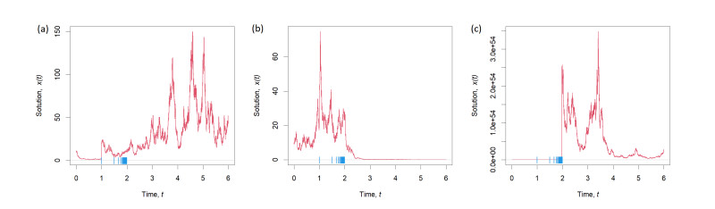
This article aims to investigate sufficient conditions for the stability of the trivial solution of stochastic differential equations with a random structure, particularly in contexts involving the presence of concentration points. The proof of asymptotic stability leverages the use of Lyapunov functions, supplemented by additional constraints on the magnitudes of jumps and jump times, as well as the Markov property of the system solutions. The findings are elucidated with an example, demonstrating both stable and unstable conditions of the system. The novelty of this work is in the consideration of jump concentration points, which are not considered in classical works. The assumption of the existence of concentration points leads to additional constraints on jumps, jump times and relations between them.
- system of random structure,
- Markov switching,
- concentration point,
- Lyapunov function,
- asymptotic stability
Citation: Taras Lukashiv, Igor V. Malyk, Maryna Chepeleva, Petr V. Nazarov. Stability of stochastic dynamic systems of a random structure with Markov switching in the presence of concentration points[J]. AIMS Mathematics, 2023, 8(10): 24418-24433. doi: 10.3934/math.20231245

Related Papers:

Abstract

This article aims to investigate sufficient conditions for the stability of the trivial solution of stochastic differential equations with a random structure, particularly in contexts involving the presence of concentration points. The proof of asymptotic stability leverages the use of Lyapunov functions, supplemented by additional constraints on the magnitudes of jumps and jump times, as well as the Markov property of the system solutions. The findings are elucidated with an example, demonstrating both stable and unstable conditions of the system. The novelty of this work is in the consideration of jump concentration points, which are not considered in classical works. The assumption of the existence of concentration points leads to additional constraints on jumps, jump times and relations between them.

References

[1]	T. Lukashiv, I. Malyk, Existence and uniqueness of solution of stochastic dynamic systems with Markov switching and concentration points, Int. J. Differ. Equ., 2017 (2017), 7958398. https://doi.org/10.1155/2017/7958398 doi: 10.1155/2017/7958398
[2]	A. P. Trofymchuk, A. P. Trofymchuk, Switching systems with fixed moments shocks the general location: Existence, uniqueness of the solution and the correctness of the Cauchy problem, Ukrainian Math. J., 42 (1990), 230–237.
[3]	E. B. Dynkin, Markov processes, Heidelberg: Springer, 1965. https://doi.org/10.1007/978-3-662-00031-1_4
[4]	B. Oksendal, Stochastic differential equation, Heidelberg: Springer, 2013. https://doi.org/10.1007/978-3-642-14394-6_5
[5]	R. Khasminskii, Stochastic stability of differential equations, Berlin: Springer, 2011.
[6]	T. Lukashiv, Y. Litvinchuk, I. V. Malyk, A. Golebiewska, P. V. Nazarov, Stabilization of stochastic dynamical systems of a random structure with Markov switchings and poisson perturbations, Mathematics, 11 (2023), 582. https://doi.org/10.3390/math11030582 doi: 10.3390/math11030582
[7]	T. O. Lukashiv, I. V. Yurchenko, V. K. Yasinskii, Lyapunov function method for investigation of stability of stochastic Ito random-structure systems with impulse Markov switchings. I. General theorems on the stability of stochastic impulse systems, Cybernet. Systems Anal., 45 (2009), 281–290. https://doi.org/10.1007/s10559-009-9102-8 doi: 10.1007/s10559-009-9102-8
[8]	M. L. Sverdan, E. F. Tsar'kov, Stability of stochastic impulse systems, Riga: RTU, 1994.
[9]	A. V. Skorokhod, Asymptotic methods in the theory of stochastic differential equations, American Mathematical Society, 2009.
[10]	J. Jacod, A. N. Shiryaev, Limit theorems for stochastic processes, Heidelberg: Springer Berlin, 2003. https://doi.org/10.1007/978-3-662-05265-5
[11]	J. L. Doob, Stochastic processes, Wiley-Interscience, 1991.
[12]	A. M. Lyapunov, General problem of stability of motion, CRC Press, 1992.
[13]	T. Lukashiv, One form of Lyapunov operator for stochastic dynamic system with Markov parameters, J. Math., 2016 (2016), 1694935. https://doi.org/10.1155/2016/1694935 doi: 10.1155/2016/1694935
[14]	I. Ya. Kats, Lyapunov function method in problems of stability and stabilization of random-structure systems, 1998.
[15]	V. K. Yasinsky, Stability in the first approximation of random-structure diffusion systems with aftereffect and external Markov switchings, Cybern. Syst. Anal., 50 (2014), 248–259. https://doi.org/10.1007/s10559-014-9612-x doi: 10.1007/s10559-014-9612-x

Reader Comments

Your name:*

Email:*
© 2023 the Author(s), licensee AIMS Press. This is an open access article distributed under the terms of the Creative Commons Attribution License (http://creativecommons.org/licenses/by/4.0)