New computations for the two-mode version of the fractional Zakharov-Kuznetsov model in plasma fluid by means of the Shehu decomposition method

Maysaa Al-Qurashi; Saima Rashid; Fahd Jarad; Madeeha Tahir; Abdullah M. Alsharif; Maysaa Al-Qurashi; Saima Rashid; Fahd Jarad; Madeeha Tahir; Abdullah M. Alsharif

doi:10.3934/math.2022117

AIMS Mathematics

2022, Volume 7, Issue 2: 2044-2060. doi: 10.3934/math.2022117

Previous Article Next Article

Research article

New computations for the two-mode version of the fractional Zakharov-Kuznetsov model in plasma fluid by means of the Shehu decomposition method

1.
Department of Mathematics, King Saud University, P. O. Box 22452, Riyadh 11495, Saudi Arabia
2.
Department of Mathematics, Government College University, Faisalabad, Pakistan
3.
Department of Mathematics, Çankaya University, Ankara, Turkey
4.
Department of Medical Research, China Medical University Hospital, China Medical University, Taichung, Taiwan
5.
Department of Mathematics, Government College Women University, Faisalabad, Pakistan
6.
Department of Mathematics, Faculty of Science, Taif University, P. O. Box 11099, Taif 21944, Saudi Arabia

Received: 06 August 2021 Accepted: 24 October 2021 Published: 05 November 2021
MSC : 26A33, 26A51, 26D07, 26D10, 26D15

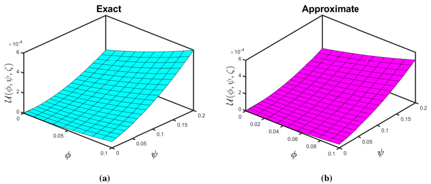
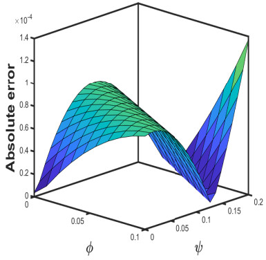
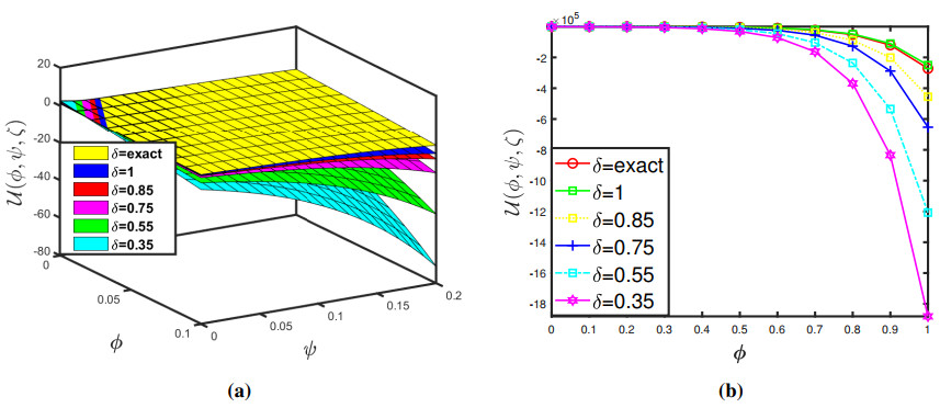
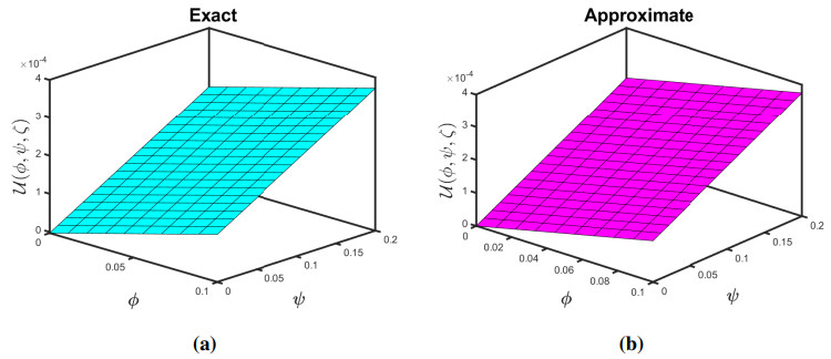
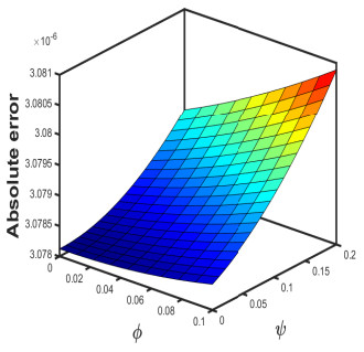
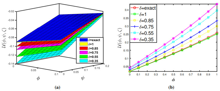
In this research, the Shehu transform is coupled with the Adomian decomposition method for obtaining the exact-approximate solution of the plasma fluid physical model, known as the Zakharov-Kuznetsov equation (briefly, ZKE) having a fractional order in the Caputo sense. The Laplace and Sumudu transforms have been refined into the Shehu transform. The action of weakly nonlinear ion acoustic waves in a plasma carrying cold ions and hot isothermal electrons is investigated in this study. Important fractional derivative notions are discussed in the context of Caputo. The Shehu decomposition method (SDM), a robust research methodology, is effectively implemented to generate the solution for the ZKEs. A series of Adomian components converge to the exact solution of the assigned task, demonstrating the solution of the suggested technique. Furthermore, the outcomes of this technique have generated important associations with the precise solutions to the problems being researched. Illustrative examples highlight the validity of the current process. The usefulness of the technique is reinforced via graphical and tabular illustrations as well as statistics theory.

Keywords:

Citation: Maysaa Al-Qurashi, Saima Rashid, Fahd Jarad, Madeeha Tahir, Abdullah M. Alsharif. New computations for the two-mode version of the fractional Zakharov-Kuznetsov model in plasma fluid by means of the Shehu decomposition method[J]. AIMS Mathematics, 2022, 7(2): 2044-2060. doi: 10.3934/math.2022117

Related Papers:

[1]	Samia Bushnaq, Sajjad Ali, Kamal Shah, Muhammad Arif . Approximate solutions to nonlinear fractional order partial differential equations arising in ion-acoustic waves. AIMS Mathematics, 2019, 4(3): 721-739. doi: 10.3934/math.2019.3.721
[2]	M. Ali Akbar, Norhashidah Hj. Mohd. Ali, M. Tarikul Islam . Multiple closed form solutions to some fractional order nonlinear evolution equations in physics and plasma physics. AIMS Mathematics, 2019, 4(3): 397-411. doi: 10.3934/math.2019.3.397
[3]	M. Hafiz Uddin, M. Ali Akbar, Md. Ashrafuzzaman Khan, Md. Abdul Haque . New exact solitary wave solutions to the space-time fractional differential equations with conformable derivative. AIMS Mathematics, 2019, 4(2): 199-214. doi: 10.3934/math.2019.2.199
[4]	Mamta Kapoor, Nehad Ali Shah, Wajaree Weera . Analytical solution of time-fractional Schrödinger equations via Shehu Adomian Decomposition Method. AIMS Mathematics, 2022, 7(10): 19562-19596. doi: 10.3934/math.20221074
[5]	Rasool Shah, Abd-Allah Hyder, Naveed Iqbal, Thongchai Botmart . Fractional view evaluation system of Schrödinger-KdV equation by a comparative analysis. AIMS Mathematics, 2022, 7(11): 19846-19864. doi: 10.3934/math.20221087
[6]	Azzh Saad Alshehry, Humaira Yasmin, Rasool Shah, Roman Ullah, Asfandyar Khan . Numerical simulation and analysis of fractional-order Phi-Four equation. AIMS Mathematics, 2023, 8(11): 27175-27199. doi: 10.3934/math.20231390
[7]	Rehana Ashraf, Saima Rashid, Fahd Jarad, Ali Althobaiti . Numerical solutions of fuzzy equal width models via generalized fuzzy fractional derivative operators. AIMS Mathematics, 2022, 7(2): 2695-2728. doi: 10.3934/math.2022152
[8]	Yunmei Zhao, Yinghui He, Huizhang Yang . The two variable (φ/φ, 1/φ)-expansion method for solving the time-fractional partial differential equations. AIMS Mathematics, 2020, 5(5): 4121-4135. doi: 10.3934/math.2020264
[9]	Aslı Alkan, Halil Anaç . The novel numerical solutions for time-fractional Fornberg-Whitham equation by using fractional natural transform decomposition method. AIMS Mathematics, 2024, 9(9): 25333-25359. doi: 10.3934/math.20241237
[10]	Naher Mohammed A. Alsafri, Hamad Zogan . Probing the diversity of kink solitons in nonlinear generalised Zakharov-Kuznetsov-Benjamin-Bona-Mahony dynamical model. AIMS Mathematics, 2024, 9(12): 34886-34905. doi: 10.3934/math.20241661

Abstract

1. Introduction

Fractional partial differential equations (PDEs) have gained prominence and recognition in recent years, owing to their verified applicability in a wide range of relatively diverse domains of science and engineering. For instance, considering the nonlinear oscillation of fractional derivatives can be employed to model earthquakes, fractional derivatives in a fluid-dynamic traffic model can be leveraged to alleviate the deficiency caused by the assumption of a continuous flow of traffic. Researchers including Coimbra, Davison and Essex, Riesz, Riemann and Liouville, Hadamard, Weyl, Jumarie, Caputo and Fabrizio, Atangana and Baleanu, Grünwald and Letnikov, Liouville and Caputo have proposed a variety of fractional operator formulations and conceptions. On the other hand, the Liouville-Caputo is the finest fractional filter. Furthermore, fractional PDEs are used to model a variety of physical phenomena, including chemical reaction and population dynamics, virology, image processing, bifurcation, thermodynamics, Levy statistics, porous media, physics, and engineering problems, (see [1-7]).

The Shehu transform (ST) was recently highlighted by Maitama and Zhao [] as an interesting integral transformation. A modification of the Laplace and Sumudu transformation is the ST. However, we can retrieve the Laplace transform by replacing $\varpi = 1$ in ST. This approach can be used to compress complex non-linear PDEs into simpler equations.

The comprehensive evaluation of numerous advanced asymptotic approaches for the exploration of solitary solutions of nonlinear PDEs, and DEs has been presented, see [9-16]. For instance, the Adomian decomposition method (ADM) [17] for obtaining seven order Sawada-Kotera equations, pseudo-spectral method (PSM) [18] for finding the numerical solution of the Laxs 7th-order KdV equation, q-homotopy analysis method (q-HAM) for finding the convergence of special PDES [19], Lie symmetry analysis (LSA) [20] for dealing with the conservation laws and exact solutions of the seventh-order time fractional Sawada-Kotera-Ito equation, Laguerre wavelets collocation method (LWCM) and Haar wavelet for the numerical solution of the Benjamina-Bona-Mohany equations [21], a new Legendre Wavelets decomposition method (NLWDM) for solving PDEs [22], discrete Adomian decomposition method (DADM) [23] for constructing numerical solution of time fractional Navier-Stokes equation.

The ZKE was built in two dimensions to demonstrate nonlinear complex phenomena such as isotope waves in a massively magnetic flux uncompressed plasma [24,25].The SDM will be implemented to develop the major objectives of this research. The time-fractional ZKE is stated as:

$\begin{eqnarray} \mathcal{D}_{\zeta}^{\delta}\mathcal{U}+a_{1}(\mathcal{U}^{\eta_{1}})_{\phi}+b_{1}(\mathcal{U}^{\eta_{2}})_{\phi\phi\phi}+b_{1}(\mathcal{U}^{\eta_{3}})_{\zeta\zeta \phi} = 0, \end{eqnarray}$

(1.1)

where $\mathcal{U} = \mathcal{U}(\phi, \psi, \zeta)$ and $\mathcal{D}_{\zeta}^{\delta}$ is the Caputo fractional derivative with order $\delta, \; 0 < \delta\leq1,$ $a_{1}$ and $b_{1}$ are arbitrary constants and $\eta_{i}, \; i = 1, 2, 3$ are integers and $\eta_{i}\neq0\; (i = 1, 2, 3)$ that demonstrates the characteristics of physical phenomena such as ion acoustic waves in a plasma consisting of cold ions and hot isothermal electrons in the framework of a balanced magnetic flux ([26,27]). In [25], for example, the ZKEs were used to investigate shallowly nonlinear isotope ripples in significantly magnetism impaired plasma in three dimensions.

In spite of the incredible improvement, the Adomian decomposition method (ADM) was contemplated by Gorge Adomian in 1980. The ADM, for example, has been effectively defined in numerous analytical structures of PDEs, especially in Burger's equation [28], time-fractional Kawahara equation [29], fuzzy heat-like and wave-like equations [30] and Lane-Emden-Fowler type equations [31]. The ADM was found to be strongly associated with a plethora of integral transforms, including ARA, Shehu, Fourier, Aboodh, Laplace and others. Presently, modified Laplace ADM [32] has been utilized to effectively resolve Volterra integral equations employing the noted numerical formulation, discrete ADM [23] has been used to solve the time-fractional Navier-Stokes equation, and Laplace ADM [33] has been considered to identify the approximate results of a fractional system of epidemic structures of a vector-borne disease, and so on.

Several of the aforesaid approaches have the disadvantage of being always stratified and necessitating a significant amount of algorithmic effort. To minimize the computing complexity and intricacy, we suggested the Shehu decomposition method (SDM), which is a composition of the ST and the decomposition method for solving the time-fractional ZKE, which is the main motivation for this research. The projected technique develops a convergent series as a solution. SDM has fewer parameters than other analytical methods. It is the preferred approach because it does not require discretion or linearization.

In this study, we first provided a fractional ZKE, followed by a description of the SDM, and then, a comparison characterization of the SDM presented with the existing methods. The graphical representations were then thoroughly explained in relation to the ZK problem. We presented an algorithm for SDM, discussed its estimation accuracy, and then showed two examples that demonstrate the effectiveness and stability of a novel approach so that their obtained simulations can be analyzed. Finally, as a part of our concluding remarks, we discussed the accumulated facts of our findings.

2. Prelude

In order to perform our research, we require various terminologies and postulate outcomes from the literature.

Definition 2.1. ([]) Shehu transform (ST) for a mapping $\mathcal{U}(\zeta)$ containing exponential order defined on the set of mappings is described as follows:

$\begin{eqnarray} \mathbf{S} = \Big\{\mathcal{U}(\zeta)|\exists\mathcal{P}, p_{1}, p_{2} > 0, \big\vert\mathcal{U}(\zeta)\big\vert < \mathcal{P}\exp(|\zeta|/p_{\jmath}), \; if\; \zeta\in(-1)^{\jmath}\times[0, \infty), \jmath = 1, 2;\big(\mathcal{P}, p_{1}, p_{2} > 0\big)\Big\}, \end{eqnarray}$

(2.1)

where $\mathcal{U}(\zeta)$ is denoted by $\mathbf{S}\big[\mathcal{U}(\zeta)\big] = \mathcal{S}(\xi, \varpi),$ is stated as

$\begin{eqnarray} \mathbf{S}\big[\mathcal{U}(\zeta)\big] = \int\limits_{0}^{\infty}\mathcal{U}(\zeta)\exp\Big(-\frac{\xi}{\varpi}\zeta\Big)d\zeta = \mathcal{S}(\xi, \varpi), \; \zeta\leq0, \; \varpi\in[\kappa_{1}, \kappa_{2}]. \end{eqnarray}$

(2.2)

The following is an example of a supportive ST:

$\begin{eqnarray} \mathbf{S}\big[\zeta^{\delta}\big] = \int\limits_{0}^{\infty}\exp\Big(-\frac{\xi}{\varpi}\zeta\Big)\zeta^{\delta}d\zeta = \Gamma(\delta+1)\Big(\frac{\varpi}{\xi}\Big)^{\delta+1}. \end{eqnarray}$

(2.3)

Definition 2.2. ([]) The inverse ST of a function $\mathcal{U}(\zeta)$ is described as

$\begin{eqnarray} \mathbf{S}^{-1}\Big[\Big(\frac{\varpi}{\xi}\Big)^{m\delta+1}\Big] = \frac{\zeta^{m\delta}}{\Gamma(m\delta+1)}, \; \; \Re(\delta) > 0, \; \; and \; m > 0. \end{eqnarray}$

(2.4)

Lemma 2.3. Consider ST of $\mathcal{U}_{1}(\zeta)$ and $\mathcal{U}_{2}(\zeta)$ are $\mathcal{P}(\xi, \varpi)$ and $\mathcal{Q}(\xi, \varpi),$ respectively [8],

$\begin{eqnarray} \mathbf{S}\big[\gamma_{1}\mathcal{U}_{1}(\zeta)+\gamma_{2}\mathcal{U}_{2}(\zeta)\big]&& = \mathbf{S}\big[\gamma_{1}\mathcal{U}_{1}(\zeta)\big]+\mathbf{S}\big[\gamma_{2}\mathcal{U}_{2}(\zeta)\big]\\&& = \gamma_{1}\mathcal{P}(\xi, \varpi)+\gamma_{2}\mathcal{Q}(\xi, \varpi), \end{eqnarray}$

(2.5)

where $\gamma_{1}$ and $\gamma_{2}$ are unspecified terms.

Lemma 2.4. ([])For order $\delta > 0,$ the Caputo fractional derivative (CFD) of ST is defined as

$\begin{eqnarray} \mathbf{S}\big[\mathcal{D}_{\zeta}^{\delta}\mathcal{U}(\zeta)\big] = \Big(\frac{\xi}{\varpi}\Big)^{\delta}\mathbf{S}\big[\mathcal{U}(\phi, \zeta)\big]-\sum\limits_{\kappa = 0}^{m-1}\Big(\frac{\xi}{\varpi}\Big)^{\delta-\kappa-1}\mathcal{U}^{(\kappa)}(\phi, 0), \; m-1\leq\delta\leq m, \; m\in\mathbb{N}. \end{eqnarray}$

(2.6)

3. Description of the SDM

Considering the nonlinear partial differential equation:

$\begin{eqnarray} \mathcal{D}_{\zeta}^{\delta}\mathcal{U}(\phi, \zeta)+\mathcal{L}\mathcal{U}(\phi, \zeta)+\check{\mathcal{N}}\mathcal{U}(\phi, \zeta) = \mathcal{F}(\phi, \zeta), \; \zeta > 0, \; 0 < \delta\leq1, \end{eqnarray}$

(3.1)

subject to the condition

$\begin{eqnarray} \mathcal{U}(\phi, 0) = \mathcal{G}(\phi), \end{eqnarray}$

(3.2)

where $\mathcal{D}_{\zeta}^{\delta} = \frac{\partial^{\delta}\mathcal{U}(\phi, \zeta)}{\partial \zeta^{\delta}}$ indicates the CFD with $0 < \delta\leq1$ while $\mathcal{L}$ and $\check{\mathcal{N}}$ are linear/nonlinear factors and the source term refers to $\mathcal{F}(\phi, \zeta).$

Implementing the ST to (3.1), and we attain

$\begin{eqnarray*} \mathbf{S}\big[\mathcal{D}_{\zeta}^{\delta}\mathcal{U}(\phi, \zeta)+\mathcal{L}\mathcal{U}(\phi, \zeta)+\check{\mathcal{N}}\mathcal{U}(\phi, \zeta)\big] = \mathbf{S}\big[\mathcal{F}(\phi, \zeta)\big]. \end{eqnarray*}$

Applying the differentiation property of ST, yields

$\begin{eqnarray} &&\frac{\xi^{\delta}}{\varpi^{\delta}}\mathcal{U}(\xi, \varpi) = \sum\limits_{\kappa = 0}^{m-1}\Big(\frac{\xi}{\varpi}\Big)^{\delta-\kappa-1}\mathcal{U}^{(\kappa)}(0)+\mathbf{S}\big[\mathcal{L}\mathcal{U}(\phi, \zeta)+\check{\mathcal{N}}\mathcal{U}(\phi, \zeta)\big]+\mathbf{S}\big[\mathcal{F}(\phi, \zeta)\big]. \end{eqnarray}$

(3.3)

Th inverse ST of (3.3) provides

$\begin{eqnarray} \mathcal{U}(\phi, \zeta) = \mathbf{S}^{-1}\bigg[\sum\limits_{\kappa = 0}^{m-1}\Big(\frac{\xi}{\varpi}\Big)^{\delta-\kappa-1}\mathcal{U}^{(\kappa)}(0)+\frac{\varpi^{\delta}}{\xi^{\delta}}\mathbf{S}\big[\mathcal{F}(\phi, \zeta)\big]\bigg]-\mathbf{S}^{-1}\bigg[\frac{\varpi^{\delta}}{\xi^{\delta}}\mathbf{S}\big[\mathcal{L}\mathcal{U}(\phi, \zeta)+\check{\mathcal{N}}\mathcal{U}(\phi, \zeta)\big]\bigg]. \end{eqnarray}$

(3.4)

The infinite series representation of SDM is denoted by the mapping $\mathcal{U}(\phi, \zeta)$ as follows:

$\begin{eqnarray} \mathcal{U}(\phi, \zeta) = \sum\limits_{m = 0}^{\infty}\mathcal{U}_{m}(\phi, \zeta). \end{eqnarray}$

(3.5)

Thus, the nonlinearity ${\check{\mathcal{N}}}(\phi, \zeta)$ can be estimated by the ADM represented as

$\begin{eqnarray} {\check{\mathcal{N}}}\mathcal{U}(\phi, \zeta) = \sum\limits_{m = 0}^{\infty}\tilde{A}_{m}(\mathcal{U}_{0}, \mathcal{U}_{1}, ...), \; m = 0, 1, ...\; , \end{eqnarray}$

(3.6)

where

$\tilde{A}_{m}(\mathcal{U}_{0}, \mathcal{U}_{1}, ...) = \frac{1}{m!}\bigg[\frac{d^{m}}{d\lambda^{m}}{\check{\mathcal{N}}}\bigg(\sum\limits_{\jmath = 0}^{\infty}\lambda^{\jmath}\mathcal{U}_{\jmath}\bigg)\bigg]_{\lambda = 0}, \; \; m > 0.$

Substituting (3.5) and (3.6) into (3.4), we have

$\begin{eqnarray} \sum\limits_{m = 0}^{\infty}\mathcal{U}_{m}(\phi, \zeta)&& = \mathcal{G}(\phi)+\tilde{\mathcal{G}}(\phi)-\mathbf{S}^{-1}\bigg[\frac{\varpi^{\delta}}{\xi^{\delta}}\mathbf{S}\big[\mathcal{L}\mathcal{U}(\phi, \zeta)+\sum\limits_{m = 0}^{\infty}\tilde{A}_{m}\big]\bigg]. \end{eqnarray}$

(3.7)

Consequently, the following is the recursive methodology for (3.7):

$\begin{eqnarray} \mathcal{U}_{0}(\phi, \zeta)&& = \mathcal{G}(\phi)+\tilde{\mathcal{G}}(\phi), \; \; m = 0, \\\mathcal{U}_{m+1}(\phi, \zeta)&& = -\mathbf{S}^{-1}\bigg[\frac{\varpi^{\delta}}{\xi^{\delta}}\mathbf{S}\big[\mathcal{L}\big(\mathcal{U}_{m}(\phi, \zeta)\big)+\sum\limits_{m = 0}^{\infty}\tilde{A}_{m}\big]\bigg], \; \; m\geq1. \end{eqnarray}$

(3.8)

4. Illustrative examples

Example 4.1. Assume the following time-dependent fractional-order Zakharov-Kuznetsov equation:

$\begin{eqnarray} \mathcal{D}_{\zeta}^{\delta}\mathcal{U}+\frac{\partial\mathcal{U}^{2}}{\partial \phi}+\frac{1}{8}\Big[\frac{\partial}{\partial \phi}\Big(\frac{\partial^{2}\mathcal{U}^{2}}{\partial \psi^{2}}\Big)+\frac{\partial^{3}\mathcal{U}^{2}}{\partial \phi^{3}}\Big] = 0, \end{eqnarray}$

(4.1)

subject to the initial condition

$\begin{eqnarray} \mathcal{U}(\phi, \psi, 0) = \frac{4}{3}\theta\sinh^{2}(\phi+\psi), \end{eqnarray}$

(4.2)

where $\theta$ is an arbitrary constant.

Proof. Applying the ST on both sides of (4.1), we find

$\begin{eqnarray} &&\mathbf{S}\Big[\frac{\partial^{\delta}\mathcal{U}}{\partial\zeta^{\delta}}\Big] = -\mathbf{S}\bigg[\frac{\partial\mathcal{U}^{2}}{\partial \phi}+\frac{1}{8}\Big[\frac{\partial}{\partial \phi}\Big(\frac{\partial^{2}\mathcal{U}^{2}}{\partial \psi^{2}}\Big)+\frac{\partial^{3}\mathcal{U}^{2}}{\partial \phi^{3}}\Big]\bigg], \\&& \Big(\frac{\xi}{\varpi}\Big)^{\delta}\mathbf{S}\big[\mathcal{U}(\phi, \psi, \zeta)\big]-\sum\limits_{\kappa = 0}^{n_{1}-1} \Big(\frac{\xi}{\varpi}\Big)^{\delta-\kappa-1}\frac{\partial^{\kappa}\mathcal{U}^{(\kappa)}(\phi, 0)}{\partial\zeta^{\kappa}} = -\mathbf{S}\bigg[\frac{\partial\mathcal{U}^{2}}{\partial \phi}+\frac{1}{8}\Big[\frac{\partial}{\partial \phi}\Big(\frac{\partial^{2}\mathcal{U}^{2}}{\partial \psi^{2}}\Big)+\frac{\partial^{3}\mathcal{U}^{2}}{\partial \phi^{3}}\Big]\bigg]. \end{eqnarray}$

(4.3)

Employing the inverse ST, we have

$\begin{eqnarray} \mathcal{U}(\phi, \psi, \zeta) = \mathbf{S}^{-1}\Bigg[ \Big(\frac{\varpi}{\xi}\Big)^{\delta}\sum\limits_{\kappa = 0}^{n_{1}-1} \Big(\frac{\xi}{\varpi}\Big)^{\delta-\kappa-1}\frac{\partial^{\kappa}\mathcal{U}^{(\kappa)}(\phi, 0)}{\partial\zeta^{\kappa}}-\Big(\frac{\varpi}{\xi}\Big)^{\delta}\mathbf{S}\bigg[\frac{\partial\mathcal{U}^{2}}{\partial \phi}+\frac{1}{8}\Big[\frac{\partial}{\partial \phi}\Big(\frac{\partial^{2}\mathcal{U}^{2}}{\partial \psi^{2}}\Big)+\frac{\partial^{3}\mathcal{U}^{2}}{\partial \phi^{3}}\Big]\bigg]\Bigg]. \end{eqnarray}$

(4.4)

It follows that

$\begin{eqnarray} &&\mathcal{U}(\phi, \psi, \zeta) = \mathbf{S}^{-1}\bigg[\frac{\varpi}{\xi}{\mathcal{U}(\phi, \psi, 0)}\bigg]-\mathbf{S}^{-1}\bigg[\Big(\frac{\varpi}{\xi}\Big)^{\delta}\mathbf{S}\bigg[\frac{\partial\mathcal{U}^{2}}{\partial \phi}+\frac{1}{8}\Big[\frac{\partial}{\partial \phi}\Big(\frac{\partial^{2}\mathcal{U}^{2}}{\partial \psi^{2}}\Big)+\frac{\partial^{3}\mathcal{U}^{2}}{\partial \phi^{3}}\Big]\bigg]\Bigg], \\&&\mathcal{U}(\phi, \psi, \zeta) = \mathbf{S}^{-1}\bigg[\frac{4}{3}\frac{\varpi}{\xi}{\theta\sinh^{2}(\phi+\psi)}\bigg]-\mathbf{S}^{-1}\bigg[\Big(\frac{\varpi}{\xi}\Big)^{\delta}\mathbf{S}\bigg[\frac{\partial\mathcal{U}^{2}}{\partial \phi}+\frac{1}{8}\Big[\frac{\partial}{\partial \phi}\Big(\frac{\partial^{2}\mathcal{U}^{2}}{\partial \psi^{2}}\Big)+\frac{\partial^{3}\mathcal{U}^{2}}{\partial \phi^{3}}\Big]\bigg]\Bigg]. \end{eqnarray}$

(4.5)

Utilizing the Shehu's decomposition method, we get

$\begin{eqnarray} \sum\limits_{\jmath = 0}^{\infty}\mathcal{U}_{\jmath}(\phi, \psi, \zeta) = \frac{4}{3}\theta\sinh^{2}(\phi+\psi)-\mathbf{S}^{-1}\Bigg[\Big(\frac{\varpi}{\xi}\Big)^{\delta}\mathbf{S}\bigg[\check{\mathcal{N}}(\mathcal{U})_{\phi}+\frac{1}{8}\Big[\check{\mathcal{N}}(\mathcal{U})_{\phi\phi\phi}+\check{\mathcal{N}}(\mathcal{U})_{\phi\psi\psi}\Big]\bigg]\Bigg], \end{eqnarray}$

(4.6)

where $\check{\mathcal{N}}(\mathcal{U})$ is the Admoian's polynomial describing nonlinear term appearing in the above mentioned equations.

$\begin{eqnarray} \check{\mathcal{N}}(\mathcal{U}) = \mathcal{U}^{2} = \sum\limits_{\jmath = 0}^{\infty}\mathcal{H}_{\jmath}(\mathcal{U}). \end{eqnarray}$

(4.7)

First few Admoian's polynomials are presented as follows:

$\begin{eqnarray*} \mathcal{H}_{0}&& = \mathcal{U}_{0}^{2}, \nonumber\\ \mathcal{H}_{1}&& = 2\mathcal{U}_{0}\mathcal{U}_{1}, \nonumber\\ \mathcal{H}_{2}&& = 2\mathcal{U}_{0}\mathcal{U}_{2}+\mathcal{U}_{1}^{2}, \nonumber\\ \mathcal{U}_{0}(\phi, \psi, \zeta)&& = \frac{4}{3}\theta\sinh^{2}(\phi+\psi), \nonumber\\ \mathcal{U}_{\jmath+1}(\phi, \psi, \zeta)&& = -\mathbf{S}^{-1}\bigg[\Big(\frac{\varpi}{\xi}\Big)^{\delta}\mathbf{S}\bigg[\bigg(\sum\limits_{\jmath = 0}^{\infty}\mathcal{H}_{\jmath}(\mathcal{U})\bigg)_{\phi}+\frac{1}{8}\bigg(\sum\limits_{\jmath = 0}^{\infty}\mathcal{H}_{\jmath}(\mathcal{U})\bigg)_{\phi\phi\phi}+\frac{1}{8}\bigg(\sum\limits_{\jmath = 0}^{\infty}\mathcal{H}_{\jmath}(\mathcal{U})\bigg)_{\phi\psi\psi}\bigg], \end{eqnarray*}$

for $\jmath = 0, 1, 2, ...$

$\begin{eqnarray*} \mathcal{U}_{1}(\phi, \psi, \zeta)&& = -\mathbf{S}^{-1}\bigg[\Big(\frac{\varpi}{\xi}\Big)^{\delta}\mathbf{S}\bigg[(\mathcal{U}_{0}^{2})_{\phi}+\frac{1}{8}(\mathcal{U}_{0}^{2})_{\phi\phi\phi}+\frac{1}{8}(\mathcal{U}_{0}^{2})_{\phi\psi\psi}\bigg]\Bigg]\nonumber\\&& = \bigg(-\frac{224}{9}\theta^{2}\sinh^{2}(\phi+\psi)\cosh(\phi+\psi)-\frac{32}{3}\theta^{2}\sinh(\phi+\psi)\cosh^{3}(\phi+\psi)\bigg)\mathbf{S}^{-1}\Big(\Big(\frac{\varpi}{\xi}\Big)^{\delta+1}\Big)\nonumber\\&& = \bigg(-\frac{224}{9}\theta^{2}\sinh^{2}(\phi+\psi)\cosh(\phi+\psi)-\frac{32}{3}\theta^{2}\sinh(\phi+\psi)\cosh^{3}(\phi+\psi)\bigg)\frac{\zeta^{\delta}}{\Gamma(\delta+1)}. \end{eqnarray*}$

Accordingly, we can derive the remaining terms as follows

$\begin{eqnarray} \mathcal{U}_{2}(\phi, \psi, \zeta)&& = -\mathbf{S}^{-1}\bigg[\Big(\frac{\varpi}{\xi}\Big)^{\delta}\mathbf{S}\bigg[(2\mathcal{U}_{0}\mathcal{U}_{1})_{\phi}+\frac{1}{8}(2\mathcal{U}_{0}\mathcal{U}_{1})_{\phi\phi\phi}+\frac{1}{8}(2\mathcal{U}_{0}\mathcal{U}_{1})_{\phi\psi\psi}\bigg]\Bigg]\\&& = \frac{128}{27}\theta^{3}\Big(1200\cosh^{6}(\phi+\psi)-2080\cosh^{4}(\phi+\psi)\\&&\quad+968\cosh^{2}(\phi+\psi)-79\Big)\frac{\zeta^{2\delta}}{\Gamma(2\delta+1)}, \end{eqnarray}$

(4.8)

$\begin{eqnarray} \mathcal{U}_{3}(\phi, \psi, \zeta)&& = -\mathbf{S}^{-1}\bigg[\Big(\frac{\varpi}{\xi}\Big)^{\delta}\mathbf{S}\bigg[(2\mathcal{U}_{0}\mathcal{U}_{2}+\mathcal{U}_{1}^{2})_{\phi}+\frac{1}{8}(2\mathcal{U}_{0}\mathcal{U}_{2}+\mathcal{U}_{1}^{2})_{\phi\phi\phi}+\frac{1}{8}(2\mathcal{U}_{0}\mathcal{U}_{2}+\mathcal{U}_{1}^{2})_{\phi\psi\psi}\bigg]\Bigg]\\&& = -\frac{2048}{81}\theta^{4}\sinh(\phi+\psi)\cosh(\phi+\psi)\Big(88, 4000\cosh^{6}(\phi+\psi)-160,200\cosh^{4}(\phi+\psi)\\&&\quad+85,170\cosh^{2}(\phi+\psi)-11,903\Big)\frac{\zeta^{3\delta}}{\Gamma(3\delta+1)}. \end{eqnarray}$

(4.9)

The approximate-analytical SDM solution is

$\begin{eqnarray} \mathcal{U}(\phi, \psi, \zeta)&& = \mathcal{U}_{0}(\phi, \psi, \zeta)+\mathcal{U}_{1}(\phi, \psi, \zeta)+\mathcal{U}_{2}(\phi, \psi, \zeta)+\mathcal{U}_{3}(\phi, \psi, \zeta)+..., \\\mathcal{U}(\phi, \psi, \zeta)&& = \frac{4}{3}\theta\sinh^{2}(\phi+\psi)-\bigg(\frac{224}{9}\theta^{2}\sinh^{2}(\phi+\psi)\cosh(\phi+\psi)\\&&\quad+\frac{32}{3}\theta^{2}\sinh(\phi+\psi)\cosh^{3}(\phi+\psi)\bigg)\frac{\zeta^{\delta}}{\Gamma(\delta+1)}+\frac{128}{27}\theta^{3}\Big(1200\cosh^{6}(\phi+\psi)\\&&\quad-2080\cosh^{4}(\phi+\psi)+968\cosh^{2}(\phi+\psi)-79\Big)\frac{\zeta^{2\delta}}{\Gamma(2\delta+1)}\\&&\quad-\frac{2048}{81}\theta^{4}\sinh(\phi+\psi)\cosh(\phi+\psi)\Big(88, 4000\cosh^{6}(\phi+\psi)-160,200\cosh^{4}(\phi+\psi)\\&&\quad+85,170\cosh^{2}(\phi+\psi)-11,903\Big)\frac{\zeta^{3\delta}}{\Gamma(3\delta+1)}+...\; . \end{eqnarray}$

(4.10)

The exact solution for $\delta = 1$ is presented by

$\begin{eqnarray} \mathcal{U}(\phi, \psi, \zeta) = \frac{4}{3}\theta\sinh^{2}(\phi+\psi-\theta\zeta). \end{eqnarray}$

(4.11)

and show the comparison results for exact, SDM, and absolute error of $\mathcal{U}_{abs} = \|\mathcal{U}^{E}-\mathcal{U}^{SDM}\|$ solution for (4.1), when $\theta = 0001$ and for various fractional orders $\delta = 0.67, \; 0.75, \; 1.$ It can be seen that the proposed method closely corresponds the exact, VIM [34], VIA [35] and RPSM [35].

Table 1. Exact

$(\mathcal{U}_{E})$ and SDM-approximate

$(\mathcal{U}_{SDM})$ solution with absolute error

$(\mathcal{U}_{abs})$ in comparison derived by VIM

$(\mathcal{U}_{VIM})$ [34], PIA

$(\mathcal{U}_{PIA})$ [35] and RPSM

$(\mathcal{U}_{RPSM})$ [35] for Example 4.1 at

$\theta = 0.001,$

$\delta = 1, \; 0.67$ and 0.75.

$\phi$	$\psi$	$\zeta$	$\mathcal{U}_{E}$	$\mathcal{U}_{SDM}$	$\mathcal{U}_{abs}$	$\mathcal{U}_{\delta=0.67}$	$\mathcal{U}_{\delta=0.75}$	$\mathcal{U}_{VIM}$ [34]
0.1	0.1	0.2	5.394 $\times10^{-5}$	5.331 $\times10^{-5}$	6.313 $\times10^{-7}$	5.341 $\times10^{-5}$	5.328 $\times10^{-5}$	5.356 $\times10^{-5}$
		0.3	7.668 $\times10^{-4}$	7.562 $\times10^{-4}$	1.055 $\times10^{-5}$	7.488 $\times10^{-4}$	7.507 $\times10^{-4}$	7.570 $\times10^{-4}$
		0.4	5.383 $\times10^{-5}$	5.308 $\times10^{-5}$	7.541 $\times10^{-7}$	5.419 $\times10^{-5}$	5.375 $\times10^{-5}$	5.410 $\times10^{-5}$
0.6	0.6	0.2	7.668 $\times10^{-4}$	7.562 $\times10^{-4}$	1.055 $\times10^{-5}$	7.488 $\times10^{-4}$	7.507 $\times10^{-4}$	7.570 $\times10^{-4}$
		0.3	7.665 $\times10^{-4}$	7.513 $\times10^{-4}$	1.522 $\times10^{-5}$	7.447 $\times10^{-4}$	7.461 $\times10^{-4}$	7.531 $\times10^{-4}$
		0.4	7.663 $\times10^{-4}$	7.468 $\times10^{-4}$	1.948 $\times10^{-5}$	7.417 $\times10^{-4}$	7.425 $\times10^{-4}$	7.501 $\times10^{-4}$
0.9	0.9	0.2	1.840 $\times10^{-3}$	1.801 $\times10^{-3}$	3.993 $\times10^{-5}$	1.772 $\times10^{-3}$	1.779 $\times10^{-3}$	1.803 $\times10^{-3}$
		0.3	1.740 $\times10^{-3}$	1.882 $\times10^{-3}$	5.803 $\times10^{-5}$	1.755 $\times10^{-3}$	1.761 $\times10^{-3}$	1.788 $\times10^{-3}$
		0.4	1.840 $\times10^{-3}$	1.765 $\times10^{-3}$	7.487 $\times10^{-5}$	1.743 $\times10^{-3}$	1.747 $\times10^{-3}$	1.775 $\times10^{-3}$

| Show Table

DownLoad: CSV

Table 2. Other comparison of the projected scheme with PIA and RPSM for Example 4.1 at

$\theta = 0.001$ having different fractional-order

$\delta = 0.67$ and

$\delta = 0.75$ .

$\phi$	$\psi$	$\zeta$	$\mathcal{U}_{PIA}$ [35]	$\mathcal{U}_{RPSM}$ [35]	$\mathcal{U}_{PIA}$ [35]	$\mathcal{U}_{RPSM}$ [35]
0.1	0.1	0.2	5.3307 $\times10^{-5}$	6.3129 $\times10^{-7}$	5.3285 $\times10^{-5}$	5.3562 $\times10^{-5}$
		0.3	5.28631 $\times10^{-5}$	5.28410 $\times10^{-5}$	5.29757 $\times10^{-5}$	5.29675 $\times10^{-5}$
		0.4	5.25777 $\times10^{-5}$	5.25897 $\times10^{-5}$	5.27039 $\times10^{-5}$	5.27119 $\times10^{-5}$
0.6	0.6	0.2	2.95493 $\times10^{-3}$	2.95185 $\times10^{-3}$	2.96356 $\times10^{-3}$	2.96251 $\times10^{-3}$
		0.3	2.92662 $\times10^{-3}$	2.92709 $\times10^{-3}$	2.93717 $\times10^{-3}$	2.93780 $\times10^{-3}$
		0.4	2.90307 $\times10^{-3}$	2.90522 $\times10^{-3}$	2.91448 $\times10^{-3}$	2.91561 $\times10^{-3}$
0.9	0.9	0.2	1.06822 $\times10^{-2}$	1.05522 $\times10^{-2}$	1.07716 $\times10^{-2}$	2.91561 $\times10^{-2}$
		0.3	1.04487 $\times10^{-2}$	1.01199 $\times10^{-2}$	1.05488 $\times10^{-2}$	1.03695 $\times10^{-2}$
		0.4	9.02777 $\times10^{-2}$	9.60606 $\times10^{-2}$	1.03736 $\times10^{-2}$	9.96743 $\times10^{-2}$

| Show Table

DownLoad: CSV

Taking $\theta = 0.005$ and $\delta = 1$ , we exhibit the approximate-analytical solution of the fractional KZEs equation up to 4 components in (a and b). Furthermore, we establish absolute errors at $\delta = 1$ for the exact-approximate solutions in the accompanying . Also, we have seen how different fractional orders perform in surface plots and 2D plots in and some $\delta_{1}\delta_{2}-slice$ (a and b) solutions are presented in 4 when $\theta = 0.005$ and $\zeta = 0.5$ . As a result of this behaviour, we might conclude that the approximation solution tends to be a precise solution. Accordingly, as the iteration increases, the absolute inaccuracy decreases. Consequently, as the number of terms grows, the SDM findings approach the exact result.

Figure 1. Numerical behavior of exact and approximate solution to the

$\mathcal{U}(\phi, \psi, \zeta)$ for Example 4.1 when the parameters are

$\theta = 0.0005, \delta = 1,$ and

$\zeta = 0.5$ .

DownLoad: Full-Size Img PowerPoint

Figure 2. Surface representation of

$\mathcal{U}(\phi, \psi, \zeta)$ absolute error plot for Example 4.1 at

$\theta = 0.005$ and

$\delta = 1$ .

DownLoad: Full-Size Img PowerPoint

Figure 3. Numerical behavior of different fractional orders to the function

$\mathcal{U}(\phi, \psi, \zeta)$ for Example 4.1 when the parameters are

$\theta = 0.05,$ and

$\zeta = 0.9$ .

DownLoad: Full-Size Img PowerPoint

The graphs in Figures 1–4 assist us to comprehend the behaviour of fractional orders when space and time scale variables fluctuate. Additionally, the findings of this study will aid scientists connected to pattern formation theory, optical designs, or mathematical modelling in comprehending the structural phenomena of the ANOVA-test. Furthermore, the efficiency of the projected method can be boosted by getting additional approximate solution expressions.

Figure 4. Numerical behavior of

$\delta_{1}\delta_{2}$ -slice solution to the

$\mathcal{U}(\phi, \psi, \zeta)$ for Example 4.1 (a) exact and (b) approximate when the parameters are

$\theta = 0.0005, \delta = 1,$ and

$\zeta = 0.5$ .

DownLoad: Full-Size Img PowerPoint

Example 4.2. Assume the following time-dependent fractional-order Zakharov-Kuznetsov equation:

$\begin{eqnarray} \mathcal{D}_{\zeta}^{\delta}\mathcal{U}+\frac{\partial\mathcal{U}^{3}}{\partial \phi}+2\Big[\frac{\partial}{\partial \phi}\Big(\frac{\partial^{2}\mathcal{U}^{3}}{\partial \psi^{2}}\Big)+\frac{\partial^{3}\mathcal{U}^{3}}{\partial \phi^{3}}\Big] = 0, \end{eqnarray}$

(4.12)

subject to the initial condition

$\begin{eqnarray} \mathcal{U}(\phi, \psi, 0) = \frac{3}{2}\theta\sinh\Big[\frac{1}{6}(\phi+\psi)\Big], \end{eqnarray}$

(4.13)

where $\theta$ is an arbitrary constant.

Proof. Applying the ST on both sides of (4.12), we find

$\begin{eqnarray} &&\mathbf{S}\Big[\frac{\partial^{\delta}\mathcal{U}}{\partial\zeta^{\delta}}\Big] = -\mathbf{S}\bigg[\frac{\partial\mathcal{U}^{3}}{\partial \phi}+2\Big[\frac{\partial}{\partial \phi}\Big(\frac{\partial^{2}\mathcal{U}^{3}}{\partial \psi^{2}}\Big)+\frac{\partial^{3}\mathcal{U}^{3}}{\partial \phi^{3}}\Big]\bigg], \\&& \Big(\frac{\xi}{\varpi}\Big)^{\delta}\mathbf{S}\big[\mathcal{U}(\phi, \psi, \zeta)\big]-\sum\limits_{\kappa = 0}^{n_{1}-1} \Big(\frac{\xi}{\varpi}\Big)^{\delta-\kappa-1}\frac{\partial^{\kappa}\mathcal{U}^{(\kappa)}(\phi, 0)}{\partial\zeta^{\kappa}} = -\mathbf{S}\bigg[\frac{\partial\mathcal{U}^{3}}{\partial \phi}+2\Big[\frac{\partial}{\partial \phi}\Big(\frac{\partial^{2}\mathcal{U}^{3}}{\partial \psi^{2}}\Big)+\frac{\partial^{3}\mathcal{U}^{3}}{\partial \phi^{3}}\Big]\bigg]. \end{eqnarray}$

(4.14)

Employing the inverse ST, we have

$\begin{eqnarray} \mathcal{U}(\phi, \psi, \zeta) = \mathbf{S}^{-1}\Bigg[ \Big(\frac{\varpi}{\xi}\Big)^{\delta}\sum\limits_{\kappa = 0}^{n_{1}-1} \Big(\frac{\xi}{\varpi}\Big)^{\delta-\kappa-1}\frac{\partial^{\kappa}\mathcal{U}^{(\kappa)}(\phi, 0)}{\partial\zeta^{\kappa}}-\Big(\frac{\varpi}{\xi}\Big)^{\delta}\mathbf{S}\bigg[\frac{\partial\mathcal{U}^{3}}{\partial \phi}+2\Big[\frac{\partial}{\partial \phi}\Big(\frac{\partial^{2}\mathcal{U}^{3}}{\partial \psi^{2}}\Big)+\frac{\partial^{3}\mathcal{U}^{3}}{\partial \phi^{3}}\Big]\bigg]\Bigg]. \end{eqnarray}$

(4.15)

It follows that

$\begin{eqnarray} &&\mathcal{U}(\phi, \psi, \zeta) = \mathbf{S}^{-1}\bigg[\frac{\varpi}{\xi}{\mathcal{U}(\phi, \psi, 0)}\bigg]-\mathbf{S}^{-1}\bigg[\Big(\frac{\varpi}{\xi}\Big)^{\delta}\mathbf{S}\bigg[\frac{\partial\mathcal{U}^{3}}{\partial \phi}+2\Big[\frac{\partial}{\partial \phi}\Big(\frac{\partial^{2}\mathcal{U}^{3}}{\partial \psi^{2}}\Big)+\frac{\partial^{3}\mathcal{U}^{3}}{\partial \phi^{3}}\Big]\bigg]\Bigg], \\&&\mathcal{U}(\phi, \psi, \zeta) = \mathbf{S}^{-1}\bigg[\frac{3}{2}\frac{\varpi}{\xi}{\theta\sinh\big[\frac{1}{6}(\phi+\psi)\big]}\bigg]-\mathbf{S}^{-1}\bigg[\Big(\frac{\varpi}{\xi}\Big)^{\delta}\mathbf{S}\bigg[\frac{\partial\mathcal{U}^{3}}{\partial \phi}+2\Big[\frac{\partial}{\partial \phi}\Big(\frac{\partial^{2}\mathcal{U}^{3}}{\partial \psi^{2}}\Big)+\frac{\partial^{3}\mathcal{U}^{3}}{\partial \phi^{3}}\Big]\bigg]\Bigg]. \end{eqnarray}$

(4.16)

Utilizing the Shehu's decomposition method, we get

$\begin{eqnarray} \sum\limits_{\jmath = 0}^{\infty}\mathcal{U}_{\jmath}(\phi, \psi, \zeta) = \frac{3}{2}\theta\sinh\big[\frac{1}{6}(\phi+\psi)\big]-\mathbf{S}^{-1}\Bigg[\Big(\frac{\varpi}{\xi}\Big)^{\delta}\mathbf{S}\bigg[\check{\mathcal{N}}(\mathcal{U})_{\phi}+\frac{1}{8}\Big[\check{\mathcal{N}}(\mathcal{U})_{\phi\phi\phi}+\check{\mathcal{N}}(\mathcal{U})_{\phi\psi\psi}\Big]\bigg]\Bigg], \end{eqnarray}$

(4.17)

where $\check{\mathcal{N}}(\mathcal{U})$ is the Admoian's polynomial describing nonlinear term appearing in the above mentioned equations.

$\begin{eqnarray} \check{\mathcal{N}}(\mathcal{U}) = \mathcal{U}^{3} = \sum\limits_{\jmath = 0}^{\infty}\mathcal{G}_{\jmath}(\mathcal{U}). \end{eqnarray}$

(4.18)

First few Admoian's polynomials are presented as follows:

$\begin{eqnarray*} \mathcal{G}_{0}&& = \mathcal{U}_{0}^{3}, \nonumber\\ \mathcal{G}_{1}&& = 3\mathcal{U}_{0}^{2}\mathcal{U}_{1}, \nonumber\\ \mathcal{G}_{2}&& = 3\mathcal{U}_{0}^{2}\mathcal{U}_{2}+3\mathcal{U}_{0}^{2}\mathcal{U}_{1}^{2}, \nonumber\\ \mathcal{U}_{0}(\phi, \psi, \zeta)&& = \frac{3}{2}\theta\sinh\Big[\frac{1}{6}(\phi+\psi)\Big], \nonumber\\ \mathcal{U}_{\jmath+1}(\phi, \psi, \zeta)&& = -\mathbf{S}^{-1}\bigg[\Big(\frac{\varpi}{\xi}\Big)^{\delta}\mathbf{S}\bigg[\bigg(\sum\limits_{\jmath = 0}^{\infty}\mathcal{G}_{\jmath}(\mathcal{U})\bigg)_{\phi}+2\bigg(\sum\limits_{\jmath = 0}^{\infty}\mathcal{G}_{\jmath}(\mathcal{U})\bigg)_{\phi\phi\phi}+2\bigg(\sum\limits_{\jmath = 0}^{\infty}\mathcal{G}_{\jmath}(\mathcal{U})\bigg)_{\phi\psi\psi}\bigg], \end{eqnarray*}$

for $\jmath = 0, 1, 2, ...$

$\begin{eqnarray*} \mathcal{U}_{1}(\phi, \psi, \zeta)&& = -\mathbf{S}^{-1}\bigg[\Big(\frac{\varpi}{\xi}\Big)^{\delta}\mathbf{S}\bigg[(\mathcal{U}_{0}^{3})_{\phi}+2(\mathcal{U}_{0}^{3})_{\phi\phi\phi}+2(\mathcal{U}_{0}^{3})_{\phi\psi\psi}\bigg]\Bigg]\nonumber\\&& = \bigg(-3\theta^{3}\sinh^{2}\Big[\frac{1}{6}(\phi+\psi)\Big]\cosh\Big[\frac{1}{6}(\phi+\psi)\Big]+\frac{3}{8}\theta^{3}\cosh^{3}\Big[\frac{1}{6}(\phi+\psi)\Big]\bigg)\mathbf{S}^{-1}\Big(\Big(\frac{\varpi}{\xi}\Big)^{\delta+1}\Big)\nonumber\\&& = \bigg(-3\theta^{3}\sinh^{2}\Big[\frac{1}{6}(\phi+\psi)\Big]\cosh\Big[\frac{1}{6}(\phi+\psi)\Big]+\frac{3}{8}\theta^{3}\cosh^{3}\Big[\frac{1}{6}(\phi+\psi)\Big]\bigg)\frac{\zeta^{\delta}}{\Gamma(\delta+1)}. \end{eqnarray*}$

Accordingly, we can derive the remaining terms as follows

$\begin{eqnarray*} \mathcal{U}_{2}(\phi, \psi, \zeta)&& = -\mathbf{S}^{-1}\bigg[\Big(\frac{\varpi}{\xi}\Big)^{\delta}\mathbf{S}\bigg[(3\mathcal{U}_{0}^{2}\mathcal{U}_{1})_{\phi}+2(3\mathcal{U}_{0}^{2}\mathcal{U}_{1})_{\phi\phi\phi}+2(3\mathcal{U}_{0}^{2}\mathcal{U}_{1})_{\phi\psi\psi}\bigg]\Bigg]\nonumber\\&& = \frac{3}{32}\theta^{5}\sinh\Big[\frac{1}{6}(\phi+\psi)\Big]\bigg[765\cosh^{4}\Big[\frac{1}{6}(\phi+\psi)\Big]\nonumber\\&&\quad-729\cosh^{2}\Big[\frac{1}{6}(\phi+\psi)\Big]+91\bigg]\frac{\zeta^{2\delta}}{\Gamma(2\delta+1)}, \end{eqnarray*}$

$\begin{eqnarray*} \mathcal{U}_{3}(\phi, \psi, \zeta)&& = -\mathbf{S}^{-1}\bigg[\Big(\frac{\varpi}{\xi}\Big)^{\delta}\mathbf{S}\bigg[(3\mathcal{U}_{0}^{2}\mathcal{U}_{2}+3\mathcal{U}_{0}^{2}\mathcal{U}_{1}^{2})_{\phi}\nonumber\\&&\quad+2(3\mathcal{U}_{0}^{2}\mathcal{U}_{2}+3\mathcal{U}_{0}^{2}\mathcal{U}_{1}^{2})_{\phi\phi\phi}+2(3\mathcal{U}_{0}^{2}\mathcal{U}_{2}+3\mathcal{U}_{0}^{2}\mathcal{U}_{1}^{2})_{\phi\psi\psi}\bigg]\Bigg]\nonumber\\&& = -\frac{3}{128}\cosh\Big[\frac{1}{6}(\phi+\psi)\Big]\bigg[171,738\cosh^{6}\Big[\frac{1}{6}(\phi+\psi)\Big]-349,884\cosh^{4}\Big[\frac{1}{6}(\phi+\psi)\Big]\nonumber\\&&\quad+215,496\cosh^{2}\Big[\frac{1}{6}(\phi+\psi)\Big]-36,907\bigg]\frac{\zeta^{3\delta}}{\Gamma(3\delta+1)}. \end{eqnarray*}$

The approximate-analytical SDM solution is

$\begin{eqnarray} \mathcal{U}(\phi, \psi, \zeta)&& = \mathcal{U}_{0}(\phi, \psi, \zeta)+\mathcal{U}_{1}(\phi, \psi, \zeta)+\mathcal{U}_{2}(\phi, \psi, \zeta)+\mathcal{U}_{3}(\phi, \psi, \zeta)+..., \\\mathcal{U}(\phi, \psi, \zeta)&& = \frac{3}{2}\theta\sinh\Big[\frac{1}{6}(\phi+\psi)\Big]-\bigg(3\theta^{3}\sinh^{2}\Big[\frac{1}{6}(\phi+\psi)\Big]\cosh\Big[\frac{1}{6}(\phi+\psi)\Big]\\&&\quad+\frac{3}{8}\theta^{3}\cosh^{3}\Big[\frac{1}{6}(\phi+\psi)\Big]\bigg)\frac{\zeta^{\delta}}{\Gamma(\delta+1)}\\&&\quad+\frac{3}{32}\theta^{5}\sinh\Big[\frac{1}{6}(\phi+\psi)\Big]\bigg[765\cosh^{4}\Big[\frac{1}{6}(\phi+\psi)\Big]-729\cosh^{2}\Big[\frac{1}{6}(\phi+\psi)\Big]\\&&\quad+91\bigg]\frac{\zeta^{2\delta}}{\Gamma(2\delta+1)}-\frac{3}{128}\cosh\Big[\frac{1}{6}(\phi+\psi)\Big]\bigg[171,738\cosh^{6}\Big[\frac{1}{6}(\phi+\psi)\Big]\\&&\quad-349,884\cosh^{4}\Big[\frac{1}{6}(\phi+\psi)\Big]\\&&\quad+215,496\cosh^{2}\Big[\frac{1}{6}(\phi+\psi)\Big]-36,907\bigg]\frac{\zeta^{3\delta}}{\Gamma(3\delta+1)}+...\; . \end{eqnarray}$

(4.19)

The exact solution for $\delta = 1$ is presented by

$\begin{eqnarray} \mathcal{U}(\phi, \psi, \zeta) = \frac{3}{2}\theta\sinh\Big[\frac{1}{6}(\phi+\psi-\theta\zeta)\Big]. \end{eqnarray}$

(4.20)

show the comparison results for exact, SDM, and absolute error of $\mathcal{U}_{abs} = \|\mathcal{U}^{E}-\mathcal{U}^{SDM}\|$ solution for (4.12), when $\theta = 0001$ and for various fractional orders $\delta = 0.67, \; 0.75, \; 1.$ It can be seen that the proposed method closely matches the exact, and VIM [34].

Table 3. Exact

$(\mathcal{U}_{E})$ and SDM-approximate

$(\mathcal{U}_{SDM})$ solution with absolute error

$(\mathcal{U}_{abs})$ in comparison derived by VIM

$(\mathcal{U}_{VIM})$ [34], for Example 4.2 at

$\theta = 0.001,$

$\delta = 1, \; 0.67$ and 0.75.

$\phi$	$\psi$	$\zeta$	$\mathcal{U}_{E}$	$\mathcal{U}_{SDM}$	$\mathcal{U}_{abs}$	$\mathcal{U}_{0.67}$	$\mathcal{U}_{0.75}$	$\mathcal{U}_{VIM}$
0.1	0.1	0.2	4.996 $\times10^{-5}$	5.001 $\times10^{-5}$	4.988 $\times10^{-8}$	5.001 $\times10^{-5}$	5.001 $\times10^{-5}$	5.001 $\times10^{-5}$
		0.3	4.993 $\times10^{-5}$	5.001 $\times10^{-5}$	7.481 $\times10^{-8}$	5.001 $\times10^{-5}$	5.001 $\times10^{-5}$	5.001 $\times10^{-5}$
		0.4	4.991 $\times10^{-5}$	5.001 $\times10^{-5}$	9.975 $\times10^{-8}$	5.001 $\times10^{-5}$	5.001 $\times10^{-5}$	5.001 $\times10^{-5}$
0.6	0.6	0.2	3.020 $\times10^{-4}$	3.020 $\times10^{-4}$	5.079 $\times10^{-8}$	3.020 $\times10^{-4}$	3.020 $\times10^{-4}$	3.020 $\times10^{-4}$
		0.3	3.019 $\times10^{-4}$	3.020 $\times10^{-4}$	7.619 $\times10^{-8}$	3.020 $\times10^{-4}$	3.020 $\times10^{-4}$	3.020 $\times10^{-4}$
		0.4	3.019 $\times10^{-4}$	3.020 $\times10^{-4}$	1.016 $\times10^{-7}$	3.020 $\times10^{-4}$	3.020 $\times10^{-4}$	3.020 $\times10^{-4}$
0.9	0.9	0.2	4.567 $\times10^{-4}$	4.568 $\times10^{-4}$	5.198 $\times10^{-8}$	4.568 $\times10^{-4}$	4.568 $\times10^{-4}$	4.568 $\times10^{-4}$
		0.3	4.567 $\times10^{-4}$	4.568 $\times10^{-4}$	7.797 $\times10^{-7}$	4.568 $\times10^{-4}$	4.568 $\times10^{-4}$	4.568 $\times10^{-4}$
		0.4	4.567 $\times10^{-4}$	4.568 $\times10^{-4}$	1.040 $\times10^{-7}$	4.568 $\times10^{-4}$	4.568 $\times10^{-4}$	4.568 $\times10^{-4}$

| Show Table

DownLoad: CSV

Taking $\theta = 0.0005$ and $\delta = 1$ , we exhibit the approximate-analytical solution of the fractional KZEs equation up to 4 components in (a and b), respectively. Furthermore, we established absolute errors at different values of $\delta$ for the exact-approximate solutions in the accompanying Figure 6. Also, we have seen how different fractional orders perform in 2D and 3D plots in in (a and b) behaves. Also, denotes the $\delta_{1}\delta_{2}$ -slice solutions for the exact and approximate solutions (a and b), respectively. As a result of this behaviour, we might conclude that the approximation solution tends to actual solution. Accordingly, as iteration increases, the absolute inaccuracy decreases. Consequently, as the iterations expands, the SDM findings approaches the exact result. The graphs in Figures 5–8 assist us to comprehend the behaviour of fractional orders when space and time scale variables fluctuate. Additionally, the findings of this study will aid scientists connecting in pattern formation theory, optical designs, or mathematical modelling in comprehending the structural phenomena of the ANOVA-test. Furthermore, the efficiency of the projected method can be boosted by getting additional approximate solution expressions.

Figure 5. Numerical behavior of exact and approximate solution to the

$\mathcal{U}(\phi, \psi, \zeta)$ for Example 4.2 when the parameters are

$\theta = 0.0005, \delta = 1,$ and

$\zeta = 0.5$ .

DownLoad: Full-Size Img PowerPoint

Figure 6. Surface representation of

$\mathcal{U}(\phi, \psi, \zeta)$ absolute error plot for Example 4.2 at

$\theta = 0.005$ and

$\delta = 1$ .

DownLoad: Full-Size Img PowerPoint

Figure 7. Numerical behavior of

$\delta_{1}\delta_{2}$ -slice solution to the

$\mathcal{U}(\phi, \psi, \zeta)$ for Example 4.2 (a) exact and (b) approximate when the parameters are

$\theta = 0.0005, \delta = 1,$ and

$\zeta = 0.5$ .

DownLoad: Full-Size Img PowerPoint

Figure 8. Numerical behavior of

$\delta_{1}\delta_{2}$ -slice solution to the

$\mathcal{U}(\phi, \psi, \zeta)$ for Example 4.1 (a) exact and (b) approximate when the parameters are

$\theta = 0.0005, \delta = 1,$ and

$\zeta = 0.5$ .

DownLoad: Full-Size Img PowerPoint

5. Conclusions

In this paper, the Shehu decomposition method (SDM) is effectively implemented for solving nonlinear time-fractional ZKEs. The proposed findings illustrate that there is a strong correlation between the projected method and the closed form solutions. Moreover, the governed approach is reliable and pragmatic for solving other diverse linear and nonlinear PDEs appearing in various disciplines of physics and mathematics. However, this methodology does not necessitate the condition matrix, Lagrange multiplier, or costly integration calculations, so the findings are noise-free, which addresses the drawbacks of earlier techniques. It is worth mentioning that the proposed methods are pragmatic analytical tools for identifying approximate-analytical solutions to complicated nonlinear PDEs. Moreover, we deduce that this approach will be used to deal with other non-linear fractional order systems of equations that are extremely complex.

Acknowledgments

This research was supported by Taif University Research Supporting Project Number (TURSP-2020/96), Taif University, Taif, Saudi Arabia.

Conflict of interest

The authors declare that they have no conflict of interest.

References

[1]	S. Kumar, A. Atangana, A numerical study of the nonlinear fractional mathematical model of tumor cells in presence of chemotherapeutic treatment, Int. J. Biomath., 13 (2020), 2050021. doi: 10.1142/S1793524520500217. doi: 10.1142/S1793524520500217
[2]	B. Ghanbari, A. Atangana, A new application of fractional Atangana-Baleanu derivatives: designing ABC-fractional masks in image processing, Physica A, 542 (2020), 123516. doi: 10.1016/j.physa.2019.123516. doi: 10.1016/j.physa.2019.123516
[3]	I. Podlubny, Fractional differential equations, Academic Press, 1999.
[4]	R. Hilfer, Applications of fractional calculus in physics, Word Scientific, 2000.
[5]	A. Kilbas, H. M. Srivastava, J. J. Trujillo, Theory and application of fractional differential equations, Elsevier, 2006.
[6]	R. L. Magin, Fractional calculus in bioengineering, Begell House, 2006.
[7]	S. G. Samko, A. A. Kilbas, O. I. Marichev, Fractional integrals and derivatives: Theory and applications, Gordon and Breach, 1993.
[8]	S. Maitama, W. Zhao, New integral transform: Shehu transform a generalization of Sumudu and Laplace transform for solving differential equations, Int. J. Anal. Appl., 17 (2019), 167–190.
[9]	S. Rashid, K. T. Kubra, S. Ullah, Fractional spatial diffusion of a biological population model via a new integral transform in the settings ofpower and Mittag–Leffler nonsingular kernel, Phys. Scr., 96 (2021), 114003. doi: 10.1088/1402-4896/ac12e5. doi: 10.1088/1402-4896/ac12e5
[10]	S. Rashid, R. Ashraf, A. O. Akdemir, M. A. Alqudah, T. Abdeljawad, M. S. Mohamed, Analytic fuzzy formulation of a time-fractional Fornberg-Whitham model with power and Mittag–Leffler kernels, Fractal Fract., 5 (2021), 113. doi: 10.3390/fractalfract5030113. doi: 10.3390/fractalfract5030113
[11]	S. Rashid, Z. Hammouch, H. Aydi, A. G. Ahmad, A. M. Alsharif, Novel computations of the time-fractional Fisher's model viageneralized fractional integral operators by means of the Elzaki transform, Fractal Fract., 5 (2021), 94. doi: 10.3390/fractalfract5030094. doi: 10.3390/fractalfract5030094
[12]	S. Rashid, K. T. Kubra, J. L. G. Guirao, Construction of an approximate analytical solution for multi-dimensional fractionalZakharov-Kuznetsov equation via Aboodh Adomian decomposition method, Symmetry, 13 (2021), 1542. doi: 10.3390/sym13081542. doi: 10.3390/sym13081542
[13]	S. S. Zhou, S. Rashid, A. Rauf, K. T. Kubra, A. M. Alsharif, Initial boundary value problems for a multi-term time fractional diffusion equation with generalized fractional derivatives in time, AIMS Mathematics, 6 (2021), 12114–12132. doi: 10.3934/math.2021703. doi: 10.3934/math.2021703
[14]	S. Rashid, F. Jarad, K. M. Abualnaja, On fuzzy Volterra-Fredholm integrodifferential equation associated with Hilfer-generalizedproportional fractional derivative, AIMS Mathematics, 6 (2021), 10920–10946. doi: 10.3934/math.2021635. doi: 10.3934/math.2021635
[15]	S. Rashid, K. T. Kubra, A. Rauf, Y. M. Chu, Y. S. Hamed, New numerical approach for time-fractional partial differential equations arising in physical system involving natural decomposition method, Phys. Scr., 96 (2021), 105204. doi: 10.1088/1402-4896/ac0bce. doi: 10.1088/1402-4896/ac0bce
[16]	M. A. Alqudah, R. Ashraf, S. Rashid, J. Singh, Z. Hammouch, T. Abdeljawad, Novel numerical investigations of fuzzy Cauchy reaction–diffusion models via generalized fuzzy fractional derivative operators, Fractal Fract., 5 (2021), 151. doi: 10.3390/fractalfract5040151. doi: 10.3390/fractalfract5040151
[17]	S. El-Sayed, D. Kaya. An application of the ADM to seven-order Sawada-Kotara equations, Appl. Math. Comput., 157 (2004), 93–101. doi: 10.1016/j.amc.2003.08.104. doi: 10.1016/j.amc.2003.08.104
[18]	M. T. Darvishia, S. Kheybaria, F. Khanib, A numerical solution of the Lax's 7th-order KdV equation by Pseudo spectral method and Darvishi's Preconditioning, Int. J. Contemp. Math. Sciences, 2 (2007), 1097–1106. doi: 10.12988/ijcms.2007.07111
[19]	M. A. El-Tawil, S. Huseen, On convergence of the q-homotopy analysis method, Int. J. Contemp. Math. Scis., 8 (2013), 481–497. doi: 10.12988/ijcms.2013.13048
[20]	M. I. El-Bahi, K. Hilal, Lie symmetry analysis, exact solutions, and conservation laws for the generalized time-fractional KdV-Like equation, J. Funct. Space., 2021 (2021), 6628130. doi: 10.1155/2021/6628130. doi: 10.1155/2021/6628130
[21]	S. C. Shiralashetti, S. Kumbinarasaiah, Laguerre wavelets collocation method for the numerical solution of the Benjamina–Bona–Mohany equations, J. Taibah Univ. Sci., 13 (2019), 9–15. doi: 10.1080/16583655.2018.1515324. doi: 10.1080/16583655.2018.1515324
[22]	N. A. Lahmar, O. Belhamitib, S. M. Bahric, A new Legendre-Wavelets decomposition method for solving PDEs, Malaya. J. Mat, 1 (2014), 72–81.
[23]	G. A. Birajdar, Numerical solution of time fractional Navier-Stokes equation by discrete Adomian decomposition method, Nonlinear Eng., 3 (2014), 21–26. doi: 10.1515/nleng-2012-0004. doi: 10.1515/nleng-2012-0004
[24]	V. E. Zakharov, E. A. Kuznetsov, Three dimensional solutions, Soviet Phys. JETP, 39 (1974), 285–286.
[25]	D. Kumara, J. Singh, S. Kumar, Numerical computation of nonlinear fractional Zakharov-Kuznetsov equation arising in ion-acoustic waves, J. Egypt. Math. Soc., 22 (2014), 373–378. doi: 10.1016/j.joems.2013.11.004. doi: 10.1016/j.joems.2013.11.004
[26]	S. Monro, E. J. Parkes, The derivation of a modified Zakharov-Kuznetsov equation and the stability of its solutions, J. Plasma Phys., 62 (1999), 305–317. doi: 10.1017/S0022377899007874. doi: 10.1017/S0022377899007874
[27]	S. Monro, E. J. Parkes, Stability of solitary-wave solutions to a modified Zakharov-Kuznetsov equation, J. Plasma Phys., 64 (2000), 411–426. doi: 10.1017/S0022377800008771. doi: 10.1017/S0022377800008771
[28]	I. P. Akpan, Adomian decomposition approach to the solution of the Burger's equation, Am. J. Comput. Math., 5 (2015), 329–335. doi: 10.4236/ajcm.2015.53030. doi: 10.4236/ajcm.2015.53030
[29]	W. Li, Y. Pang, Application of Adomian decomposition method to nonlinear systems, Adv. Differ. Equ., 2020 (2020), 67. doi: 10.1186/s13662-020-2529-y. doi: 10.1186/s13662-020-2529-y
[30]	M. Osman, Z. Gong, A. M. Mustafa, Comparison of fuzzy Adomian decomposition method with fuzzy VIM for solving fuzzy heat-like and wave-like equations with variable coefficients, Adv. Differ. Equ., 2020 (2020), 327. doi: 10.1186/s13662-020-02784-w. doi: 10.1186/s13662-020-02784-w
[31]	A. M. Wazwaz, R. Rach, L. Bougoffa, J. S. Duan, Solving the Lane-Emden-Fowler type equations of higher orders by the Adomian decomposition method, Comput. Model. Eng. Sci., 100 (2014), 507–529.
[32]	D. Rani, V. Mishra, Modification of Laplace Adomian decomposition method for solving nonlinear Volterra integral and integro-differential equations based on Newton Raphson formula, Eur. J. Pure. Appl. Math., 11 (2018), 202–214. doi: 10.29020/nybg.ejpam.v11i1.2645. doi: 10.29020/nybg.ejpam.v11i1.2645
[33]	F. Haq, K. Shah, A. Khan, M. Shahzad, Numerical solution of fractional order epidemic model of a vector born disease by Laplace Adomian decomposition method, Punjab Univ. J. Math., 49 (2017), 13–22.
[34]	R. Y. Molliq, M. S. M. Noorani, I. Hashim, R. R. Ahmad, Approximate solutions of fractional Zakharov-Kuznetsov equations by VIM, J. Comput. Appl. Math., 233 (2009), 103–108. doi: 10.1016/j.cam.2009.03.010. doi: 10.1016/j.cam.2009.03.010
[35]	M. Şenol, M. Alquran, H. D. Kasmaei, On the comparison of perturbation-iteration algorithm and residual power series method to solve fractional Zakharov-Kuznetsov equation, Results Phys., 9 (2018), 321–327. doi: 10.1016/j.rinp.2018.02.056. doi: 10.1016/j.rinp.2018.02.056

This article has been cited by:

1.	Mostafa M.A. Khater, Thongchai Botmart, Unidirectional shallow water wave model; Computational simulations, 2022, 42, 22113797, 106010, 10.1016/j.rinp.2022.106010
2.	Alina Alb Lupas, Characteristics of a Subclass of Analytic Functions Introduced by Using a Fractional Integral Operator, 2022, 8, 2409-5761, 75, 10.15377/2409-5761.2021.08.5
3.	Maysaa Al Qurashi, Saima Rashid, Sobia Sultana, Fahd Jarad, Abdullah M. Alsharif, Fractional-order partial differential equations describing propagation of shallow water waves depending on power and Mittag-Leffler memory, 2022, 7, 2473-6988, 12587, 10.3934/math.2022697
4.	Mostafa M. A. Khater, Computational Traveling Wave Solutions of the Nonlinear Rangwala–Rao Model Arising in Electric Field, 2022, 10, 2227-7390, 4658, 10.3390/math10244658
5.	Vediyappan Govindan, Samad Noeiaghdam, Unai Fernandez-Gamiz, Sagar Ningonda Sankeshwari, R. Arulprakasam, Bing Zhao Li, Shehu Integral Transform and Hyers-Ulam Stability of nth order Linear Differential Equations, 2022, 18, 24682276, e01427, 10.1016/j.sciaf.2022.e01427
6.	Rashid Nawaz, Nicholas Fewster-Young, Nek Muhammad Katbar, Nasir Ali, Laiq Zada, Rabha W. Ibrahim, Wasim Jamshed, Haifa Alqahtani, Numerical inspection of (3 + 1)- perturbed Zakharov–Kuznetsov equation via fractional variational iteration method with Caputo fractional derivative, 2024, 85, 1040-7790, 1162, 10.1080/10407790.2023.2262123
7.	M. L. Rupa, K. Aruna, K. Raghavendar, Insights into the time Fractional Belousov-Zhabotinsky System Arises in Thermodynamics, 2024, 63, 1572-9575, 10.1007/s10773-024-05770-0
8.	Saumya Ranjan Jena, Itishree Sahu, A novel approach for numerical treatment of traveling wave solution of ion acoustic waves as a fractional nonlinear evolution equation on Shehu transform environment, 2023, 98, 0031-8949, 085231, 10.1088/1402-4896/ace6de
9.	Yong Zhang, Graham E. Fogg, HongGuang Sun, Donald M. Reeves, Roseanna M. Neupauer, Wei Wei, Adjoint subordination to calculate backward travel time probability of pollutants in water with various velocity resolutions, 2024, 28, 1607-7938, 179, 10.5194/hess-28-179-2024

Reader Comments

Your name:*

Email:*
© 2022 the Author(s), licensee AIMS Press. This is an open access article distributed under the terms of the Creative Commons Attribution License (http://creativecommons.org/licenses/by/4.0)

通讯作者: 陈斌, bchen63@163.com

1.
沈阳化工大学材料科学与工程学院沈阳 110142

AIMS Mathematics

1.8 3.4

Metrics

Article views(2377) PDF downloads(126) Cited by(9)

Preview PDF

Download XML

Export Citation

Article outline

Show full outline

Figures and Tables

Figures(8) / Tables(3)

AIMS Mathematics

New computations for the two-mode version of the fractional Zakharov-Kuznetsov model in plasma fluid by means of the Shehu decomposition method

Related Papers:

Abstract

1. Introduction

2. Prelude

3. Description of the SDM

4. Illustrative examples

5. Conclusions

Acknowledgments

Conflict of interest

References

This article has been cited by:

Reader Comments

通讯作者: 陈斌, bchen63@163.com

Metrics

Figures and Tables

Other Articles By Authors

Catalog

AIMS Mathematics

New computations for the two-mode version of the fractional Zakharov-Kuznetsov model in plasma fluid by means of the Shehu decomposition method

Related Papers:

Abstract

1. Introduction

2. Prelude

3. Description of the SDM

4. Illustrative examples

5. Conclusions

Acknowledgments

Conflict of interest

References

This article has been cited by:

Reader Comments

通讯作者: 陈斌, bchen63@163.com

Metrics

Figures and Tables

Other Articles By Authors

Related pages

Tools

Export File

Citation

Format

Content

Catalog