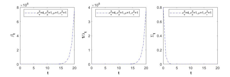
In this paper, the insider trading model of Xiao and Zhou (Acta Mathematicae Applicatae, 2021) is further studied, in which market makers receive partial information about a static risky asset and an insider stops trading at a random time. With the help of dynamic programming principle, we obtain a unique linear Bayesian equilibrium consisting of insider's trading intensity and market liquidity parameter, instead of none Bayesian equilibrium as before. It shows that (i) as time goes by, both trading intensity and market depth increase exponentially, while residual information decreases exponentially; (ii) with average trading time increasing, trading intensity decrease, but both residual information and insider's expected profit increase, while market depth is a unimodal function with a unique minimum with respect to average trading time; (iii) the less information observed by market makers, the weaker trading intensity and market depth are, but the more both expect profit and residual information are, which is in accord with our economic intuition.
Citation: Kai Xiao, Yonghui Zhou. Linear Bayesian equilibrium in insider trading with a random time under partial observations[J]. AIMS Mathematics, 2021, 6(12): 13347-13357. doi: 10.3934/math.2021772
In this paper, the insider trading model of Xiao and Zhou (Acta Mathematicae Applicatae, 2021) is further studied, in which market makers receive partial information about a static risky asset and an insider stops trading at a random time. With the help of dynamic programming principle, we obtain a unique linear Bayesian equilibrium consisting of insider's trading intensity and market liquidity parameter, instead of none Bayesian equilibrium as before. It shows that (i) as time goes by, both trading intensity and market depth increase exponentially, while residual information decreases exponentially; (ii) with average trading time increasing, trading intensity decrease, but both residual information and insider's expected profit increase, while market depth is a unimodal function with a unique minimum with respect to average trading time; (iii) the less information observed by market makers, the weaker trading intensity and market depth are, but the more both expect profit and residual information are, which is in accord with our economic intuition.

| [1] |
K. Aase, T. Bjuland, B. Øksendal, Strategic insider trading equilibrium: A filter theory approach, Afr. Mat., 23 (2012), 145–162. doi: 10.1007/s13370-011-0026-x

|
| [2] |
K. Back, Insider trading in continuous time, Rev. Financ. Stud., 5 (1992), 387–409. doi: 10.1093/rfs/5.3.387
|
| [3] |
K. Back, H. Pedersen, Long-lived information and intraday patterns, J. Financ. Mark., 1 (1998), 385–402. doi: 10.1016/S1386-4181(97)00003-7
|
| [4] |
F. Biagini, Y. Hu, T. Myer-Brandis, B. Øksendal, Insider trading equilibrium in a market with memory, Math. Finan. Econ., 6 (2012), 229–247. doi: 10.1007/s11579-012-0065-6
|
| [5] | R. Caldentey, E. Stacchetti, Insider trading with a random deadline, Econometrica, 1 (2010), 245–283. |
| [6] |
L. Campi, U. Cetin, A. Danilova, Dynamic Markov bridges motivated by models of insider trading, Stoch. Proc. Appl., 121 (2011), 534–567. doi: 10.1016/j.spa.2010.11.004
|
| [7] |
L. Campi, U. Cetin, Insider trading in an equilibrium model with default: A passage from reduced-form to structral modelling, Financ. Stoch., 11 (2007), 591–602. doi: 10.1007/s00780-007-0038-4
|
| [8] |
K. Cho, Continuous auctions and insider trading, Financ. Stoch., 7 (2003), 47–71. doi: 10.1007/s007800200078
|
| [9] | P. Collins-Dufresne, V. Fos, Insider trading, stochastic liquidity and equilibrium prices, Econometrica, 84 (2016), 1451–1475. |
| [10] |
F. Fostor, S. Viswanathan, Strategic trading when agents forecast the forcasts of others, J. Finance, 51 (1996), 1437–1478. doi: 10.1111/j.1540-6261.1996.tb04075.x
|
| [11] |
A. Kyle, Continuous auctions and insider trading, Econometrica, 53 (1985), 1315–1335. doi: 10.2307/1913210
|
| [12] | R. Liptser, A. Shiryaev, Statistics of Random Processes: General Theory, Springer, 2001. |
| [13] | R. Liptser, A. Shiryaev, Statistics of Random Processes II. Applications, Springer, 2001. |
| [14] |
S. Luo, The impact of public information on insider trading, Econ. Lett., 70 (2001), 59–68. doi: 10.1016/S0165-1765(00)00347-5
|
| [15] |
J. Ma, R. Sun, Y. Zhou, Kyle-Back equilibrium models and linear conditional mean-field SDEs, SIAM J. Control Optim., 56 (2018), 1154–1180. doi: 10.1137/15M102558X
|
| [16] | K. Xiao, Y. Zhou, Insider trading with a random deadline under partial observations: Maximal principle method, Accepted by Acta Math. Appl. Sin-E., 2021. |
| [17] | J. Yong, X. Zhou, Stochastic Controls, Springer, 2012. |
| [18] |
Y. Zhou, Existence of linear strategy equilibrium in insider trading with partial observations, J. Sys. Sci. Complex., 29 (2016), 1–12. doi: 10.1007/s11424-015-4074-4
|


Figures(3)

Kai Xiao, Yonghui Zhou. Linear Bayesian equilibrium in insider trading with a random time under partial observations[J]. AIMS Mathematics, 2021, 6(12): 13347-13357. doi: 10.3934/math.2021772


 DownLoad: