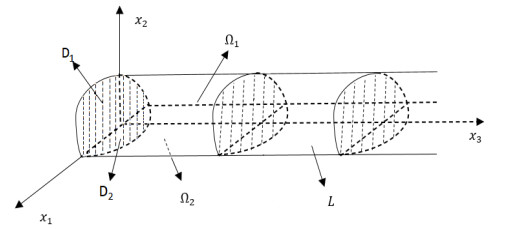
Spatial decay estimates for the Fochheimer equations interfacing with a Darcy equations

Ze Wang; Yan Zhang; Jincheng Shi; Baiping Ouyang; Ze Wang; Yan Zhang; Jincheng Shi; Baiping Ouyang

doi:10.3934/math.2021728

AIMS Mathematics

2021, Volume 6, Issue 11: 12632-12649. doi: 10.3934/math.2021728

Previous Article Next Article

Research article

Spatial decay estimates for the Fochheimer equations interfacing with a Darcy equations

1.
Department of Computer Science, Guangdong University of Finance, Yingfu Road, Guangzhou 510521, China
2.
Department of Public Infrastructure, Guangdong Teachers College of Foreign Language and Arts, Longdong East Road, Guangzhou 510521, China
3.
Department of Applied Mathematics, Guangzhou Huashang College, Huashang Road, Guangzhou 511300, China

Received: 02 August 2021 Accepted: 27 August 2021 Published: 02 September 2021
MSC : 35B30, 35K55, 35Q35

Spatial decay estimates for the Fochheimer fluid interfacing with a Darcy flow in a semi-infinite pipe was studied. The exponential decay result can be obtained by integrating a first-order differential inequality. The result can be seen as the usage of Saint-Venant's principle for the interfacing fluids.
- Saint-Venant's principle,
- decay estimates,
- Forchheimer fluid,
- Darcy fluid
Citation: Ze Wang, Yan Zhang, Jincheng Shi, Baiping Ouyang. Spatial decay estimates for the Fochheimer equations interfacing with a Darcy equations[J]. AIMS Mathematics, 2021, 6(11): 12632-12649. doi: 10.3934/math.2021728

Related Papers:

Abstract

Spatial decay estimates for the Fochheimer fluid interfacing with a Darcy flow in a semi-infinite pipe was studied. The exponential decay result can be obtained by integrating a first-order differential inequality. The result can be seen as the usage of Saint-Venant's principle for the interfacing fluids.

References

[1]	B. A. Boley, The determination of temperature, stresses and deflection in two-dimensional thermoelastic problem, J. Aero. Sci., 23 (1956), 67–75. doi: 10.2514/8.3503
[2]	C. O. Horgan, J. K. Knowles, Recent developments concerning Saint-Venant's principle, Adv. Appl. Mech., 23 (1983), 179–264. doi: 10.1016/S0065-2156(08)70244-8
[3]	C. O. Horgan, Recent developments concerning Saint-Venant's principle: An update, Appl. Mech. Rev., 42 (1989), 295–302. doi: 10.1115/1.3152414
[4]	C. O. Horgan, Recent development concerning Saint-Venant's principle: A second update, Appl. Mech. Rev., 49 (1996), s101–s111. doi: 10.1115/1.3101961
[5]	B. Straughan, Mathematical aspects of penetrative convection, CRC Press, 1993.
[6]	P. N. Kaloni, J. Guo, Double diffusive convection in a porous medium, nonlinear stability and the Brinkman effect, Stud. Appl. Math., 94 (1995), 341–358. doi: 10.1002/sapm1995943341
[7]	J. Guo, Y. Qin, Steady nonlinear double-diffusive convection in a porous medium base upon the Brinkman-Forchheimer model, J. Math. Anal. Appl., 204 (1996), 138–155. doi: 10.1006/jmaa.1996.0428
[8]	P. N. Kaloni, Y. Qin, Spatial decay estimates for flow in the Brinkman-Forchheimer model, Quartely Appl. Math., 56 (1998), 71–87. doi: 10.1090/qam/1604880
[9]	L. E. Payne, B. Straughan, Stability in the initial-time geometry problem for the Brinkman and Darcy equations of flow in porous media, J. Math. Pures Appl., 75 (1996), 225–271.
[10]	L. E. Payne, B. Straughan, Convergence and continuous dependence for the Brinkman- Forchheimer equations, Stud. Appl. Math., 102 (1999), 419–439. doi: 10.1111/1467-9590.00116
[11]	L. E. Payne, B. Straughan, Structural stability for the Darcy equations of flow in porous media, P. Roy. Soc. A, 54 (1984), 1691–1698.
[12]	L. E. Payne, J. C. Song, B. Straughan, Continuous dependence and convergence results for Brinkman and Forchheimer models with variable viscosity, P. Roy. Soc. A, 45 (1999), 2173–2190.
[13]	K. A. Ames, L. E. Payne, Continuous dependence results for an ill-posed problem in nonlinear viscoelasticity, Z. Angew. Math. Phys., 48 (1997), 20–29. doi: 10.1007/PL00001467
[14]	F. Franchi, B. Straughan, Structural stability for the Brinkman equations of porous media, Math. Methods Appl. Sci., 19 (1996), 1335–1347. doi: 10.1002/(SICI)1099-1476(19961110)19:16<1335::AID-MMA842>3.0.CO;2-Y
[15]	K. A. Ames, L. E. Payne, On stabilizing against modeling errors in a penetrative convection problem for a porous medium, Math. Mod. Methods Appl. Sci., 4 (1994), 733–740. doi: 10.1142/S0218202594000406
[16]	F. Franchi, Stabilization estimates for penetrative motions in porous media, Math. Methods Appl. Sci., 17 (1994), 11–20. doi: 10.1002/mma.1670170103
[17]	A. Morro, B. Straughan, Continuous dependence on the source parameters for convective motion in porous media, Nonlinear Anal.: Theory Methods Appl., 18 (1992), 307–315. doi: 10.1016/0362-546X(92)90147-7
[18]	Y. Qin, P. N. Kaloni, Steady convection in a porous medium based upon the Brinkman model, IMA J. Appl. Math., 48 (1992), 85–95. doi: 10.1093/imamat/48.1.85
[19]	L. Richardson, B. Straughan, Convection with temperature dependent viscosity in a porous medium: Nonlinear stability and the Brinkman effect, Atti Accad. Naz. Lincei, Cl. Sci. Fisiche, Mat. Nat., Rend. Lincei, Mat. Appl., 4 (1993), 223–230.
[20]	L. E. Payne, J. C. Song, Spatial decay bounds for double diffusive convection in Brinkman flow, J. Differ. Equations, 244 (2008), 413–430. doi: 10.1016/j.jde.2007.10.003
[21]	W. Liu, J. T. Cui, Z. F. Wang, Numerical analysis and modeling of multiscale Forchheimer-Forchheimer coupled model for compressible fluid flow in fractured media aquifer system, Appl. Math. Comput., 353 (2019), 7–28.
[22]	J. S. Kou, S. Y. Sun, Y. Q. Wu, A semi-analytic porosity evolution scheme for simulating wormhole propagation with the Darcy-Brinkman-Forchheimer model, J. Comput. Appl. Math., 348 (2019), 401–420. doi: 10.1016/j.cam.2018.08.055
[23]	Y. Liu, S. Z. Xiao, Structural stability for the Brinkman fluid interfacing with a Darcy fluid in an unbounded domain, Nonlinear Anal.: Real World Appl., 42 (2018), 308–333. doi: 10.1016/j.nonrwa.2018.01.007
[24]	A. K. Alzahrani, Darcy-Forchheimer 3D flow of carbon nanotubes with homogeneous and heterogeneous reactions, Phys. Lett. A, 382 (2018), 2787–2793. doi: 10.1016/j.physleta.2018.06.011
[25]	Y. Liu, Continuous dependence for a thermal convection model with temperature-dependent solubility, Appl. Math. Comput., 308 (2017), 18–30.
[26]	F. A. Morales, R. E. Showalter, A Darcy-Brinkman model of fractures in porous media, J. Math. Anal. Appl., 452 (2017), 1332–1358. doi: 10.1016/j.jmaa.2017.03.063
[27]	Y. F. Li, C. H. Lin, Continuous dependence for the nonhomogeneous Brinkman-Forchheimer equations in a semi-infinite pipe, Appl. Math. Comput., 244 (2014), 201–208.
[28]	N. L. Scott, Continuous dependence on boundary reaction terms in a porous medium of Darcy type, J. Math. Anal. Appl., 399 (2013), 667–675. doi: 10.1016/j.jmaa.2012.10.054
[29]	B. Jamil, M. S. Anwar, A. Rasheeda, M. Irfanc, MHD Maxwell flow modeled by fractional derivatives with chemical reaction and thermal radiation, Chin. J. Phys., 67 (2020), 512–533. doi: 10.1016/j.cjph.2020.08.012
[30]	M. S. Anwar, R. T. M. Ahmad, T. Shahzad, M. Irfanc, M. Z. Ashraf, Electrified fractional nanofluid flow with suspended carbon nanotubes, Comput. Math. Appl., 80 (2020), 1375–1386. doi: 10.1016/j.camwa.2020.07.005
[31]	M. S. Anwar, Numerical study of transport phenomena in a nanofluid using fractional relaxation times in Buongiorno model, Phys. Scr., 95 (2020), 035211. doi: 10.1088/1402-4896/ab4ba9
[32]	M. Irfan, M. S. Anwar, M. Rashid, M. Waqas, W. A. Khan, Arrhenius activation energy aspects in mixed convection Carreau nanofluid with nonlinear thermal radiation, Appl. Nanosci., 10 (2020), 4403–4413. doi: 10.1007/s13204-020-01498-5
[33]	M. S. Anwar, A. Rasheed, Joule heating in magnetic resistive flow with fractional Cattaneo-Maxwell model, J. Braz. Soc. Mech. Sci. Eng., 40 (2018), 501. doi: 10.1007/s40430-018-1426-8
[34]	M. S. Anwar, A. Rasheed, Interplay of chemical reacting species in a fractional viscoelastic fluid flow, J. Mol. Liq., 273 (2019), 576–588. doi: 10.1016/j.molliq.2018.10.028
[35]	M. Farooq, M. Javed, M. Ijaz Khan, A. Anjum, T. Hayat, Melting heat transfer and double stratification in stagnation flow of viscous nanofluid, Results Phys., 7 (2017), 2297–2301.
[36]	M. Ijaz Khan, M. Waqas, T. Hayat, A. Al-saedi, Magneto-hydrodynamical numerical simulation of heat transfer in MHD stagnation point flow of Cross fluid model towards a stretched surface, Phys. Chem. Liq., 56 (2018), 584–595. doi: 10.1080/00319104.2017.1367791
[37]	K. A. Ames, L. E. Payne, J. C. Song, Spatial decay in the pipe flow of a viscous fluid interfacing a porous medium, Math. Mod. Methods Appl. Sci., 11 (2001), 1547–1562. doi: 10.1142/S021820250100146X
[38]	G. Mckay, B. Straughan, Patterned ground formation under water, Contin. Mech. Thermodyn., 5 (1993), 145–162.
[39]	D. A. Nield, A. Bejan, Convection in porous media, Springer-Verlag, 2006.
[40]	L. E. Payne, B. Straughan, Analysis of the boundary condition at the interface between a viscous fluid and a porous medium and related questions, J. Math. Pures Appl., 77 (1998), 317–354. doi: 10.1016/S0021-7824(98)80102-5
[41]	Y. F. Li, S. H. Zhang, C. H. Lin, Structural stability for the Boussinesq equations interfacing with Darcy equations in a bounded domain, Bound. Value Probl., 2021 (2021), 27. doi: 10.1186/s13661-021-01501-0
[42]	Y. Liu, S. Z. Xiao, Y. W. Lin, Continuous dependence for the Brinkman-Forchheimer fluid interfacing with a Darcy fluid in a bounded domain, Math. Comput. Simulat., 150 (2018), 66–82. doi: 10.1016/j.matcom.2018.02.009
[43]	Y. Liu, S. Z. Xiao, Structural stability for the Brinkman fluid interfacing with a Darcy fluid in an unbounded domain, Nonlinear Anal.: Real World Appl., 42 (2018), 308-333.
[44]	J. C. Shi, Y. Liu, Structural stability for the Forchheimer equations interfacing with a Darcy fluid in a bounded region in $R^3$, Bound. Value Probl., 2021 (2021), 46.
[45]	Y. Liu, X. L. Qin, J. C. Shi, W. J. Zhi, Structural stability of the Boussinesq fluid interfacing with a Darcy fluid in a bounded region in $R^2$, Appl. Math. Comput., 411 (2021), 126488.
[46]	L. E. Payne, J. C. Song, Spatial decay estimates for Brinkman and Darcy flows in a semi-infinite cylinder, Continuum Mech. Therm., 9 (1997), 175–190. doi: 10.1007/s001610050064
[47]	Y. X. Li, T. Muhammad, M. Bilal, M. A. Khan, A. Ahmadian, B. A. Pansera, Fractional simulation for Darcy-Forchheimer hybrid nanoliquid flow with partial slip over a spinning disk, Alexandria Eng. J., 60 (2021), 4787–4796. doi: 10.1016/j.aej.2021.03.062
[48]	M. Z. Ullah, T. Muhammad, F. Mallawi, On model for Darcy-Forchheimer 3D nanofluid flow subject to heat flux boundary condition, J. Therm. Anal. Calorim., 143 (2021), 2411–2418. doi: 10.1007/s10973-020-09892-5
[49]	H. Waqas, M. Imran, T. Muhammad, S. M. Sait, R. Ellahi, On bio-convection thermal radiation in Darcy-Forchheimer flow of nanofluid with gyrotactic motile microorganism under Wu's slip over stretching cylinder/plate, Int. J. Numer. Methods Heat Fluid Flow, 31 (2021), 1520–1546. doi: 10.1108/HFF-05-2020-0313
[50]	H. Rout, S. S. Mohapatra, S. Shaw, T. Muhammad, M. K. Nayak, O. D. Makinde, Entropy optimization for Darcy-Forchheimer electro-magneto-hydrodynamic slip flow of ferronanofluid due to stretching/shrinking rotating disk, Waves Random Complex Media, 2021. Available from: https://doi.org/10.1080/17455030.2021.1927238.
[51]	M. Ijaz Khan, Transportation of hybrid nanoparticles in forced convective Darcy-Forchheimer flow by a rotating disk, Int. Commun. Heat Mass Transfer, 122 (2021), 105177. doi: 10.1016/j.icheatmasstransfer.2021.105177
[52]	M. Ijaz Khan, F. Alzahrani, A. Hobiny, Simulation and modeling of second order velocity slip flow of micropolar ferrofluid with Darcy-Forchheimer porous medium, J. Mater. Res. Technol., 9 (2020), 7335–7340. doi: 10.1016/j.jmrt.2020.04.079
[53]	T. Muhammad, K. Rafique, M. Asma, M. Alghamdi, Darcy-Forchheimer flow over an exponentially stretching curved surface with Cattaneo-Christov double diffusion, Phys. A: Stat. Mech. Appl., 556 (2020), 123968. doi: 10.1016/j.physa.2019.123968
[54]	L. E. Payne, J. C. Song, Spatial decay bounds for the Forchheimer equations, Int. J. Eng. Sci., 40 (2002), 943–956. doi: 10.1016/S0020-7225(01)00102-1

Reader Comments

Your name:*

Email:*
© 2021 the Author(s), licensee AIMS Press. This is an open access article distributed under the terms of the Creative Commons Attribution License (http://creativecommons.org/licenses/by/4.0)