Existence and global behavior of the solution to a parabolic equation with nonlocal diffusion

Fengfei Jin; Baoqiang Yan; Fengfei Jin; Baoqiang Yan

doi:10.3934/math.2021313

AIMS Mathematics

2021, Volume 6, Issue 5: 5292-5315. doi: 10.3934/math.2021313

Previous Article Next Article

Research article

Existence and global behavior of the solution to a parabolic equation with nonlocal diffusion

Fengfei Jin ,
Baoqiang Yan ^,

School of Mathematics and Statistics, Shandong Normal University, Jinan 250014, China

Received: 09 December 2020 Accepted: 22 February 2021 Published: 12 March 2021
MSC : 35K57, 35B35

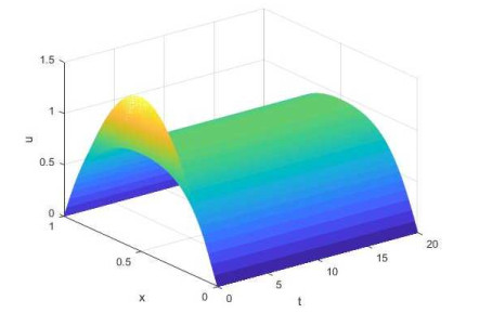
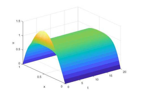
In this paper, we are concerned with the existence, uniqueness and long-time behavior of the solutions for a parabolic equation with nonlocal diffusion even if the reaction term is not Lipschitz-continuous at $ 0 $ and grows superlinearly or exponentially at $ +\infty $. First, we give a special sub-supersolution pair for some parabolic equations with nonlocal diffusion and establish the method of sub-supersolution. Second, using the sub-supersolution method, we prove the existence, uniqueness and long-time behavior of positive solutions. Finally, some one-dimensional numerical experiments are presented.
- parabolic equation with nonlocal diffusion,
- sub-supersolution method, existence,
- uniqueness,
- long-time behavior
Citation: Fengfei Jin, Baoqiang Yan. Existence and global behavior of the solution to a parabolic equation with nonlocal diffusion[J]. AIMS Mathematics, 2021, 6(5): 5292-5315. doi: 10.3934/math.2021313

Related Papers:

Abstract

In this paper, we are concerned with the existence, uniqueness and long-time behavior of the solutions for a parabolic equation with nonlocal diffusion even if the reaction term is not Lipschitz-continuous at $ 0 $ and grows superlinearly or exponentially at $ +\infty $. First, we give a special sub-supersolution pair for some parabolic equations with nonlocal diffusion and establish the method of sub-supersolution. Second, using the sub-supersolution method, we prove the existence, uniqueness and long-time behavior of positive solutions. Finally, some one-dimensional numerical experiments are presented.

References

[1]	A. S. Ackleh, L. Ke, Existence-uniqueness and long time behavior for a class of nonlocal nonlinear parabolic evolution equations, Proc. Am. Math. Soc., 128 (2000), 3483-3492. doi: 10.1090/S0002-9939-00-05912-8
[2]	R. A. Adams, Sobolev Spaces, New York: Academic Press, 1975.
[3]	R. M. P. Almeida, S. N. Antontsev, J. C. M. Duque, On a nonlocal degenerate parabolic problem, Nonlinear Anal.: Real World Appl., 27 (2016), 146-157. doi: 10.1016/j.nonrwa.2015.07.015
[4]	R. M. P. Almeida, S. N. Antontsev, J. C. M. Duque, J. Ferreira, A reaction-diffusion model for the non-local coupled system: Existence, uniqueness, long-time behaviour and localization properties of solutions, IMA J. Appl. Math., 81 (2016), 344-364. doi: 10.1093/imamat/hxv041
[5]	C. O. Alves, D. P. Covei, Existence of solution for a class of nonlocal elliptic problem via sub-supersolution method, Nonlinear Anal.: Real World Appl., 23 (2015), 1-8. doi: 10.1016/j.nonrwa.2014.11.003
[6]	T. Caraballo, M. H. Cobos, P. M. Rubio, Long-time behavior of a non-autonomous parabolic equation with nonlocal diffusion and sublinear terms, Nonlinear Anal., 121 (2015), 3-18 doi: 10.1016/j.na.2014.07.011
[7]	H. Chen, R. Yuan, Existence and stability of traveling waves for Leslie-Gower predator-prey system with nonlocal diffusion, Discrete Contin. Dyn. Syst., 37 (2017), 5433-5454. doi: 10.3934/dcds.2017236
[8]	M. Chipot, B. Lovat, Some remarks on nonlocal elliptic and parabolic problems, Nonlinear Anal., 30 (1997), 4619-4627. doi: 10.1016/S0362-546X(97)00169-7
[9]	C. De Coster, Existence and localization of solution for second order elliptic BVP in presence of lower and upper solutions without any order, J. Differ. Equations, 145 (1998), 420-452. doi: 10.1006/jdeq.1998.3423
[10]	L. Gu, Second Order Parabolic Partial Differential Equations, Xiamen: Xiamen University Press, 1995.
[11]	X. Li, S. Song, Stabilization of delay systems: Delay-dependent impulsive control, IEEE Trans. Autom. Control, 62 (2017), 406-411. doi: 10.1109/TAC.2016.2530041
[12]	X. Li, J. Wu, Stability of nonlinear differential systems with state-dependent delayed impulses, Automatica, 64 (2016), 63-69. doi: 10.1016/j.automatica.2015.10.002
[13]	Y. Liu, D. O'Regan, Controllability of impulsive functional differential systems with nonlocal conditions, Electron. J. Differ. Equations, 194 (2013), 1-10.
[14]	Y. Liu, H. Yu, Bifurcation of positive solutions for a class of boundary value problems of fractional differential inclusions, Abstr. Appl. Anal., 2013 (2013), 942831.
[15]	Y. Liu, Positive solutions using bifurcation techniques for boundary value problems of fractional differential equations, Abstr. Appl. Anal., 2013 (2013), 162418.
[16]	Y. Liu, Bifurcation techniques for a class of boundary value problems of fractional impulsive differential equations, J. Nonlinear Sci. Appl., 8 (2015), 340-353.
[17]	A. Pazy, Semigroups of Linear Operators and Applications to Partial Differential Equations, New York: Springer-Verlag, 1983.
[18]	M. H. Protter, H. F. Weinberger, Maximum Principles in Differential Equations, New York: Springer-Verlag, 1984.
[19]	C. A. Raposo, M. Sepúlveda, O. V. Villagrán, D. C. Pereira, M. L. Santos, Solution and asymptotic behaviour for a nonlocal coupled system of reaction-diffusion, Acta Applicandae Math., 102 (2008), 37-56. doi: 10.1007/s10440-008-9207-5
[20]	J. Shi, M. Yao, On a singular nonlinear semilinear elliptic problem, Proc. R. Soc. Edinburgh, Sect. A: Math., 128 (1998), 1389-1401. doi: 10.1017/S0308210500027384
[21]	Y. Sun, S. Wu, Y. Long, Combined effects of singular and superlinear nonlinearities in some singular boundary value problems, J. Differ. Equations, 176 (2001), 511-531. doi: 10.1006/jdeq.2000.3973
[22]	K. Taira, Analytic Semigroups and Semilinear Initial Boundary Value Problems, New York: Cambridge University Press, 1995.
[23]	B. Yan, T. Ma, The existence and multiplicity of positive solutions for a class of nonlocal elliptic problems, Boundary Value Probl., 165 (2016), 1-35.
[24]	B. Yan, D. O'Regan, R. P. Agarwal, The existence of positive solutions for Kirchhoff-type problems via the sub-supersolution method, An. Univ. Ovidius Constanta, Ser. Mat., 26 (2018), 5-41.
[25]	B. Yan, D. O'Regan, R. P. Agarwal, On spectral asymptotics and bifurcation for some elliptic equations of Kirchhoff-type with odd superlinear term, J. Appl. Anal. Comput., 8 (2018), 509-523.
[26]	B. Yan, D. Wang, The multiplicity of positive solutions for a class of nonlocal elliptic problem, J. Math. Anal. Appl., 442 (2016), 72-102. doi: 10.1016/j.jmaa.2016.04.023
[27]	Q. Ye, Z. Li, An Introduction to Reaction Diffusion Equations, Beijing: Science Press, 1980.
[28]	Z. Zhang, J. Yu, On a singular nonlinear Dirichlet problem with a convection term, SIAM J. Math. Anal., 32 (2000), 916-927. doi: 10.1137/S0036141097332165
[29]	Z. Zhang, K. Perera, Sign changing solutions of Kirchhoff type problems via invariant sets of descent flow, J. Math. Anal. Appl., 317 (2006), 456-463. doi: 10.1016/j.jmaa.2005.06.102
[30]	S. Zheng, M. Chipot, Asymptotic behavior of solutions to nonlinear parabolic equations with nonlocal terms, Asymptotic Anal., 45 (2005), 301-312.

Reader Comments

Your name:*

Email:*
© 2021 the Author(s), licensee AIMS Press. This is an open access article distributed under the terms of the Creative Commons Attribution License (http://creativecommons.org/licenses/by/4.0)