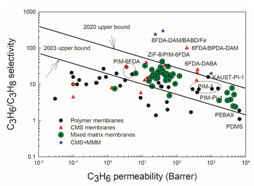
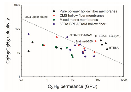
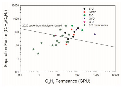
Propylene/propane separations are generally performed by distillation which are energy intensive and costly to build and operate. There is therefore high interest to develop new separation technologies like membrane modules. In our previous paper, we collected, analyzed and reported data for neat polymers and mixed matrix membranes (MMM) based on flat and hollow fiber configurations for propylene/propane separations. In this second part, we collected the data for carbon molecular sieving (CMS) membranes from polymer pyrolysis reaction and metal-organic framework (MOF) membranes from different fabrication methods, as well as data on facilitated transport membrane-polymer electrolyte membranes (PEM). CMS membranes show great potential for C3H6/C3H8 separation with an optimum pyrolysis temperature around 500–600 ℃. However, physical aging is a concern as the micro-pores shrink over time leading to lower permeability. The performance of MOF membranes are above the 2020 upper bound of polymer-based membranes, but have limited commercial application because they are fragile and difficult to produce. Finally, facilitated transport membranes show excellent propylene/propane separation performance, but are less stable compared to commercial polymeric membranes limiting their long-term operation and practical applications. As usual, there is no universal membrane and the selection must be made based on the operating conditions.
Citation: Xiao Yuan Chen, Anguo Xiao, Denis Rodrigue. Polymer based membranes for propylene/propane separation: CMS, MOF and polymer electrolyte membranes[J]. AIMS Materials Science, 2022, 9(2): 184-213. doi: 10.3934/matersci.2022012
Propylene/propane separations are generally performed by distillation which are energy intensive and costly to build and operate. There is therefore high interest to develop new separation technologies like membrane modules. In our previous paper, we collected, analyzed and reported data for neat polymers and mixed matrix membranes (MMM) based on flat and hollow fiber configurations for propylene/propane separations. In this second part, we collected the data for carbon molecular sieving (CMS) membranes from polymer pyrolysis reaction and metal-organic framework (MOF) membranes from different fabrication methods, as well as data on facilitated transport membrane-polymer electrolyte membranes (PEM). CMS membranes show great potential for C3H6/C3H8 separation with an optimum pyrolysis temperature around 500–600 ℃. However, physical aging is a concern as the micro-pores shrink over time leading to lower permeability. The performance of MOF membranes are above the 2020 upper bound of polymer-based membranes, but have limited commercial application because they are fragile and difficult to produce. Finally, facilitated transport membranes show excellent propylene/propane separation performance, but are less stable compared to commercial polymeric membranes limiting their long-term operation and practical applications. As usual, there is no universal membrane and the selection must be made based on the operating conditions.

| [1] | Chen XY, A Xiao A, Rodrigue D (2021) Polymer-based membranes for propylene/propane separation. Sep Purif Rev (in press). https://doi.org/10.1080/15422119.2021.1874415 |
| [2] |
Ren YX, Liang X, Dou HZ, et al. (2020) Membrane-based olefin/paraffin separations. Adv Sci 7: 2001398. https://doi.org/10.1002/advs.202001398 doi: 10.1002/advs.202001398

|
| [3] |
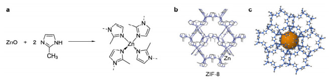
Eum K, Ma C, Rownaghi A, et al. (2016) ZIF-8 Membranes via interfacial microfluidic processing in polymeric hollow fibers: Efficient propylene separation at elevated pressures. ACS Appl Mater Inter 8: 25337-25342. https://doi.org/10.1021/acsami.6b08801 doi: 10.1021/acsami.6b08801
|
| [4] |
Eum K, Ma C, Koh DY, et al. (2017) Zeolitic imidazolate framework membranes supported on macroporous carbon hollow fibers by fluidic processing techniques. Adv Mater Interfaces 4: 1700080. https://doi.org/10.1002/admi.201700080 doi: 10.1002/admi.201700080
|
| [5] |
Koros WJ, Zhang C (2017) Materials for next-generation molecularly selective synthetic membranes. Nat Mater 16: 289-297. https://doi.org/10.1038/nmat4805 doi: 10.1038/nmat4805
|
| [6] |
Zhou HC, Long JR, Yaghi OM (2012) Introduction to metal-organic frameworks. Chem Rev 112: 673-674. https://doi.org/10.1021/cr300014x doi: 10.1021/cr300014x
|
| [7] |
Hara N, Yoshimunea M, Negishi H, et al. (2014) Diffusive separation of propylene/propane with ZIF-8 membranes. J Membrane Sci 450: 215-223. https://doi.org/10.1016/j.memsci.2013.09.012 doi: 10.1016/j.memsci.2013.09.012
|
| [8] |
Zhou HX, Zwanzig R (1991) A rate process with an entropy barrier. J Chem Phys 94: 6147-6152. https://doi.org/10.1063/1.460427 doi: 10.1063/1.460427
|
| [9] |
Kim JH, Won J, Kang YS (2004) Olefin-induced dissolution of silver salts physically dispersed in inert polymers and their applications to olefin/paraffin separation. J Membrane Sci 241: 403-407. https://doi.org/10.1016/j.memsci.2004.05.027 doi: 10.1016/j.memsci.2004.05.027
|
| [10] |
Zarca R, Ortiz A, Gorri D, et al. (2017) A practical approach to fixed-site-carrier transport modeling for the separation of propylene/propane mixtures through silver containing polymeric membranes. Sep Purif Technol 180: 82-89. https://doi.org/10.1016/j.seppur.2017.02.050 doi: 10.1016/j.seppur.2017.02.050
|
| [11] |
Hou J, Liu P, Jiang M, et al. (2019) Olefin/paraffin separation through membranes: from mechanisms to critical materials. J Mater Chem A 7: 23489-23511. https://doi.org/10.1039/C9TA06329C doi: 10.1039/C9TA06329C
|
| [12] |
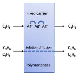
Kim JH, Kang YS, Won J (2004) Silver polymer electrolyte membranes for facilitated olefin transport: carrier properties, transport mechanism and separation performance. Macromol Res 12: 145-55. https://doi.org/10.1007/BF03218383 doi: 10.1007/BF03218383
|
| [13] |
Xu L, Rungta M, Brayden MK, et al. (2012) Olefins-selective asymmetric carbon molecular sieve hollow fiber membranes for hybrid membrane-distillation processes for olefin/paraffin separations. J Membrane Sci 423: 314-323. https://doi.org/10.1016/j.memsci.2012.08.028 doi: 10.1016/j.memsci.2012.08.028
|
| [14] |
Swaidan RJ, Ma XH, Pinnau I (2016) Spirobisindane-based polyimide as efficient precursor of thermally rearranged and carbon molecular sieve membranes for enhanced propylene/propane separation. J Membrane Sci 520: 983-989. https://doi.org/10.1016/j.memsci.2016.08.057 doi: 10.1016/j.memsci.2016.08.057
|
| [15] |
Fuertes AB, Menendez I (2002) Separation of hydrocarbon gas mixtures using phenolic resin-based carbon membranes. Sep Purif Technol 28: 29-41. https://doi.org/10.1016/S1383-5866(02)00006-0 doi: 10.1016/S1383-5866(02)00006-0
|
| [16] |
Kiyono M, Williams PJ, Koros WJ (2010) Effect of pyrolysis atmosphere on separation performance of carbon molecular sieve membranes. J Membrane Sci 359: 2-10. https://doi.org/10.1016/j.memsci.2009.10.019 doi: 10.1016/j.memsci.2009.10.019
|
| [17] |
Suda H, Haraya K (1997) Alkene/alkane permselectivities of a carbon molecular sieve membrane. Chem Commun 1: 93-94. https://doi.org/10.1039/a606385c doi: 10.1039/a606385c
|
| [18] |
Steel KM, Koros WJ (2003) Investigation of porosity of carbon materials and related effects on gas separation properties. Carbon 41: 253-266. https://doi.org/10.1016/S0008-6223(02)00309-3 doi: 10.1016/S0008-6223(02)00309-3
|
| [19] |
Steel KM, Koros WJ (2005) An investigation of the effects of pyrolysis parameters on gas separation properties of carbon materials. Carbon 43: 1843-1856. https://doi.org/10.1016/j.carbon.2005.02.028 doi: 10.1016/j.carbon.2005.02.028
|
| [20] |
Xu L, Rungta M, Koros WJ (2011) MatrimidⓇ derived carbon molecular sieve hollow fiber membranes for ethylene/ethane separation. J Membrane Sci 380: 138-147. https://doi.org/10.1016/j.memsci.2011.06.037 doi: 10.1016/j.memsci.2011.06.037
|
| [21] |
Bhuwania N, Labreche Y, Achoundong CSK, et al. (2014) Engineering substructure morphology of asymmetric carbon molecular sieve hollow fiber membranes. Carbon 76: 417-434. https://doi.org/10.1016/j.carbon.2014.05.008 doi: 10.1016/j.carbon.2014.05.008
|
| [22] |
Yerzhankyzy A, Ghanem BS, Wang Y, et al. (2020) Gas separation performance and mechanical properties of thermally-rearranged polybenzoxazoles derived from an intrinsically microporous dihydroxyl-functionalized triptycene diamine-based polyimide. J Membrane Sci 595: 117512. https://doi.org/10.1016/j.memsci.2019.117512 doi: 10.1016/j.memsci.2019.117512
|
| [23] |
Smith ZP, Hernandez G, Gleason KL (2015) Effect of polymer structure on gas transport properties of selected aromatic polyimides, polyamides and TR polymers. J Membrane Sci 493: 766-781. https://doi.org/10.1016/j.memsci.2015.06.032 doi: 10.1016/j.memsci.2015.06.032
|
| [24] |
Karunaweera C, Musselman Jr IH, Balkus KJ (2019) Fabrication and characterization of aging resistant carbon molecular sieve membranes for C3 separation using high molecular weight crosslinkable polyimide, 6FDA-DABA. J Membrane Sci 581: 430-438. https://doi.org/10.1016/j.memsci.2019.03.065 doi: 10.1016/j.memsci.2019.03.065
|
| [25] |
Okamoto K, Kawamura S, Yoshino M, et al. (1999) Olefin/paraffin separation through carbonized membranes derived from an asymmetric polyimide hollow fiber membrane. Ind Eng Chem Res 38: 4424-4432. https://doi.org/10.1021/ie990209p doi: 10.1021/ie990209p
|
| [26] |
Askari M, Yang T, Chung TS (2012) Natural gas purification and olefin/paraffin separation using cross-linkable dual-layer hollow fiber membranes comprising β-Cyclodextrin. J Membrane Sci 423-424: 392-403. https://doi.org/10.1016/j.memsci.2012.08.036 doi: 10.1016/j.memsci.2012.08.036
|
| [27] |
Hayashi J, Mizuta H, Yamamoto M, et al. (1996) Separation of ethane/ethylene and propane/propylene systems with a carbonized BPDA-p, p'-ODA polyimide membrane. Ind Eng Chem Res 35: 4176-4181. https://doi.org/10.1021/ie960264n doi: 10.1021/ie960264n
|
| [28] |
Ma XL, Lin BK, Wei XT (2013) Gamma-alumina supported carbon molecular sieve membrane for propylene/propane separation. Ind Eng Chem Res 52: 4297-4305. https://doi.org/10.1021/ie303188c doi: 10.1021/ie303188c
|
| [29] |
Ma XL, Williams S, Wei XT, et al. (2015) Propylene/propane mixture separation characteristics and stability of carbon molecular sieve membranes. Ind Eng Chem Res 54: 9824-9831. https://doi.org/10.1021/acs.iecr.5b02721 doi: 10.1021/acs.iecr.5b02721
|
| [30] | Xu LR, Rungta M, Hessleret J, al. (2014) Physical aging in carbon molecular sieve membranes. Carbon 80: 155-166. https://doi.org/10.1016/j.carbon.2014.08.051 |
| [31] |
Kim SJ, Lee PS, Chang JS, et al. (2018) Preparation of carbon molecular sieve membranes on low-cost alumina hollow fibers for use in C3H6/C3H8 separation. Sep Purif Technol 194: 443-450. https://doi.org/10.1016/j.seppur.2017.11.069 doi: 10.1016/j.seppur.2017.11.069
|
| [32] |
Ma X, Lin YS, Wei X, et al. (2016) Ultrathin carbon molecular sieve membrane for propylene/propane separation. AIChE J 62: 491-499. https://doi.org/10.1002/aic.15005 doi: 10.1002/aic.15005
|
| [33] |
Teixeira M, Campo MC, Tanaka DAP, et al. (2011) Composite phenolic resin-based carbon molecular sieve membranes for gas separation. Carbon 49: 4348-4358. https://doi.org/10.1016/j.carbon.2011.06.012 doi: 10.1016/j.carbon.2011.06.012
|
| [34] |
Qiu WL, Vaughn J, Liu GP, et al. (2019) Hyperaging tuning of a carbon molecular-sieve hollow fiber membrane with extraordinary gas-separation performance and stability. Angew Chem Int Ed 58: 11700-11703. https://doi.org/10.1002/anie.201904913 doi: 10.1002/anie.201904913
|
| [35] |
Qiu WL, Xu L, Liu Z, et al. (2021) Surprising olefin/paraffin separation performance recovery of highly aged carbon molecular sieve hollow fiber membranes by a super-hyperaging treatment. J Membrane Sci 620: 118701. https://doi.org/10.1016/j.memsci.2020.118701 doi: 10.1016/j.memsci.2020.118701
|
| [36] |
Guo M, Kanezashi M, Nagasawa H, et al. (2020) Pore subnano-environment engineering of organosilica membranes for highly selective propylene/propane separation. J Membrane Sci 60: 117999. https://doi.org/10.1016/j.memsci.2020.117999 doi: 10.1016/j.memsci.2020.117999
|
| [37] |
Guo M, Kanezashi M, Nagasawa H, et al. (2020) Fine-tuned, molecular-composite, organosilica membranes for highly efficient propylene/propane separation via suitable pore size. AIChE J 66: e16850. https://doi.org/10.1002/aic.16850 doi: 10.1002/aic.16850
|
| [38] |
Chu YH, Yancey D, Xu L, et al. (2018) Iron-containing carbon molecular sieve membranes for advanced olefin/paraffin separations. J Membrane Sci 548: 609-620. https://doi.org/10.1016/j.memsci.2017.11.052 doi: 10.1016/j.memsci.2017.11.052
|
| [39] |
Shin JH, Yu HJ, Park J, et al. (2020) Fluorine-containing polyimide/polysilsesquioxane carbon molecular sieve membranes and techno-economic evaluation thereof for C3H6/C3H8 separation. J Membrane Sci 598: 117660. https://doi.org/10.1016/j.memsci.2019.117660 doi: 10.1016/j.memsci.2019.117660
|
| [40] |
Mundstock A, Wang N, Friebe S (2015) Propane/propene permeation through Na-X membranes: The interplay of separation performance and pre-synthetic support functionalization. Micropor Mesopor Mat 215: 20-28. https://doi.org/10.1016/j.micromeso.2015.05.019 doi: 10.1016/j.micromeso.2015.05.019
|
| [41] |
André V, Quaresma S, Ferreira da Silva JL, et al. (2017) Exploring mechanochemistry to turn organic bio-relevant molecules into metal-organic frameworks: a short review. Beilstein J Org Chem 13: 2416-2427. https://doi.org/10.3762/bjoc.13.239 doi: 10.3762/bjoc.13.239
|
| [42] |
Katsenis AD, Puškarić, A, Štrukil V, et al. (2015) In situ X-ray diffraction monitoring of a mechanochemical reaction reveals a unique topology metal-organic framework. Nat Commun 6: 1-8. http://doi.org/:10.1038/ncomms7662 doi: 10.1038/ncomms7662
|
| [43] | Available from: http://www.chemtube3d.com. 2022. |
| [44] |
Pan Y, Li T, Lestari G, et al. (2012) Effective separation of propylene/propane binary mixtures by ZIF-8 membranes. J Membrane Sci 390-391: 93-98. https://doi.org/10.1016/j.memsci.2011.11.024 doi: 10.1016/j.memsci.2011.11.024
|
| [45] |
Pan Y, Liu W, Zhao Y, et al. (2015) Improved ZIF-8 membrane: Effect of activation procedure and determination of diffusivities of light hydrocarbons. J Membrane Sci 493: 88-96. https://doi.org/10.1016/j.memsci.2015.06.019 doi: 10.1016/j.memsci.2015.06.019
|
| [46] |
Liu C, Ma D, Xi X, et al. (2014) Gas transport properties and propylene/propane separation characteristics of ZIF-8 membranes. J Membrane Sci 451: 85-93. https://doi.org/10.1016/j.memsci.2013.09.029 doi: 10.1016/j.memsci.2013.09.029
|
| [47] |
Eum K, Ma C, Rownaghi A, et al. (2016) ZIF-8 membranes via interfacial microfluidic processing in polymeric hollow fibers: Efficient propylene separation at elevated pressures. ACS Appl Mater Interf 8: 25337-25342. https://doi.org/10.1021/acsami.6b08801 doi: 10.1021/acsami.6b08801
|
| [48] |
Eum K, Rownaghi A, Choi D, et al. (2016) Fluidic processing of high-performance ZIF-8 membranes on polymeric hollow fibers: Mechanistic insights and microstructure control. Adv Funct Mater 26: 5001-5018. https://doi.org/10.1002/adfm.201601550 doi: 10.1002/adfm.201601550
|
| [49] |
Zhou S, Wei Y, Li L, et al. (2018) Paralyzed membrane: Current-driven synthesis of a metal-organic framework with sharpened propene/propane separation. Sci Adv 4: 1393. https://doi.org/10.1126/sciadv.aau1393 doi: 10.1126/sciadv.aau1393
|
| [50] |
Wei R, Chi HY, Li X, et al. (2020) Aqueously cathodic deposition of ZIF-8 membranes for superior propylene/propane separation. Adv Funct Mater 30: 1907089. https://doi.org/10.1002/adfm.201907089 doi: 10.1002/adfm.201907089
|
| [51] |
Li W, Su P, Li Z, et al. (2017) Ultrathin metal-organic framework membrane production by gel-vapour deposition. Nat Commun 8: 406. https://doi.org/10.1038/s41467-017-00544-1 doi: 10.1038/s41467-017-00544-1
|
| [52] |
Ma X, Kumar P, Mittal N, et al. (2018) Zeolitic imidazolate framework membranes made by ligand-induced permselectivation. Science 361: 1008-1011. https://doi.org/10.1126/science.aat4123 doi: 10.1126/science.aat4123
|
| [53] |
Kwon HT, Jeong HK, Lee AS, et al. (2015) Heteroepitaxially grown zeolitic imidazolate framework membranes with unprecedented propylene/propane separation performances. J Am Chem Soc 137: 12304-12311. https://doi.org/10.1021/jacs.5b06730 doi: 10.1021/jacs.5b06730
|
| [54] |
Ramua G, Leea MJ, Jeong HK (2018) Effects of zinc salts on the microstructure and performance of zeoliticimidazolate framework ZIF-8 membranes for propylene/propane separation. Micropor Mesopor Mat 259: 155-162. https://doi.org/10.1016/j.micromeso.2017.10.010 doi: 10.1016/j.micromeso.2017.10.010
|
| [55] |
Kwon HY, Jeong HK (2013) In situ synthesis of thin zeolitic-imidazolate framework ZIF-8 membranes exhibiting exceptionally high propylene/propane separation. J Am Chem Soc 135: 10763-10768. https://doi.org/10.1021/ja403849c doi: 10.1021/ja403849c
|
| [56] |
Brown AJ, Brunelli NA, Eum K, et al. (2014) Interfacial microfluidic processing of metal-organic framework hollow fiber membranes. Science 345: 72-75. https://doi.org/10.1126/science.1251181 doi: 10.1126/science.1251181
|
| [57] |
Hou Q, Zhou S, Wei Y, et al. (2020) Balancing the grain boundary structure and the framework flexibility through bimetallic metal-organic framework (MOF) membranes for gas separation. JACS 142: 9582-9586. https://doi.org/10.1021/jacs.0c02181 doi: 10.1021/jacs.0c02181
|
| [58] |
Zhao Y, Wei Y, Lyu L, et al. (2020) Flexible polypropylene-supported ZIF-8 membranes for highly efficient propene/propane separation. JACS 142: 20915-20919. https://doi.org/10.1021/jacs.0c07481 doi: 10.1021/jacs.0c07481
|
| [59] |
Liu Y, Chen ZJ, Liu GP (2019) Conformation-controlled molecular sieving effects for membrane-based propylene/propane separation. Adv Mater 31: 1807513. https://doi.org/10.1002/adma.201807513 doi: 10.1002/adma.201807513
|
| [60] |
Fallanza M, Ortiz A, Gorri D, et al. (2012) Experimental study of the separation of propane/propylene mixtures by supported ionic liquid membranes containing Ag+-RTILs as carrier. Sep Purif Technol 97: 83-89. https://doi.org/10.1016/j.seppur.2012.01.044 doi: 10.1016/j.seppur.2012.01.044
|
| [61] |
Kang SW, Char K, Kang YS (2008) Novel application of partially charged silver nanoparticles for transport in olefin/paraffin separation membranes. Chem Mater 20: 1308-1311. https://doi.org/10.1021/cm071516l doi: 10.1021/cm071516l
|
| [62] |
Hsiue GH, Yang JS (1993) Novel methods in separation of olefin/paraffin mixtures by functional polymeric membranes. J Membrane Sci 82: 117-128. https://doi.org/10.1016/0376-7388(93)85097-G doi: 10.1016/0376-7388(93)85097-G
|
| [63] |
Pinnau I, Toy LG (2001) Solid polymer electrolyte composite membranes for olefin/paraffin separation. J Membrane Sci 184: 39-48. https://doi.org/10.1016/S0376-7388(00)00603-7 doi: 10.1016/S0376-7388(00)00603-7
|
| [64] |
Kang SW, Kim JH, Oh KS, et al. (2004) Highly stabilized silver polymer electrolytes and their application to olefin transport membranes. J Membrane Sci 236: 163-169. https://doi.org/10.1016/j.memsci.2004.02.020 doi: 10.1016/j.memsci.2004.02.020
|
| [65] |
Kim JH, Min B, Won J, et al. (2006) Effect of the polymer matrix on the formation of silver nanoparticles in polymer-silver salt complex membranes. J Polym Sci Pol Phys 44: 1168-1178. https://doi.org/10.1002/polb.20777 doi: 10.1002/polb.20777
|
| [66] |
Pollo LD, Durate LT, Anacleo M, et al. (2012) Polymeric membranes containing silver salts for propylene/propane separation. Brazil J Chem Eng 29: 307-314. https://doi.org/10.1590/S0104-66322012000200011 doi: 10.1590/S0104-66322012000200011
|
| [67] |
Liao KS, Lai JY, Chung TS (2016) Metal ion-modified PIM-1 and its application for propylene/propane separation. J Membrane Sci 515: 36-44. https://doi.org/10.1016/j.memsci.2016.05.032 doi: 10.1016/j.memsci.2016.05.032
|
| [68] |
Wang Y, Ren J, Deng M (2011) Ultrathin solid polymer electrolyte PEI/Pebax2533/AgBF4 composite membrane for propylene/propane separation. Sep Purif Technol 77: 46-52. https://doi.org/10.1016/j.seppur.2010.11.018 doi: 10.1016/j.seppur.2010.11.018
|
| [69] |
Kang SW, Bae W, Kim JH, et al. (2009) Behavior of inorganic nanoparticles in silver polymer electrolytes and their effects on silver ion activity for olefin transport. Ind Eng Chem Res 48: 8650-8654. https://doi.org/10.1021/ie9000103 doi: 10.1021/ie9000103
|
| [70] |
Kang SW, Kim JH, Won J, et al. (2013) Suppression of silver ion reduction by Al(NO3)3 complex and its application to highly stabilized olefin transport membranes. J Membrane Sci 445: 156. https://doi.org/10.1016/j.memsci.2013.06.010 doi: 10.1016/j.memsci.2013.06.010
|
| [71] |
Sun HX, Ma C, Wang T, et al. (2014) Satellite TiO2 nanoparticles induced by silver ion in polymer electrolytes membrane for propylene/propane separation. Mater Chem Phys 148: 790-797. https://doi.org/10.1016/j.matchemphys.2014.08.050 doi: 10.1016/j.matchemphys.2014.08.050
|
| [72] |
Park YS, Chun S, Kang YS, et al. (2017) Durable poly(vinyl alcohol)/AgBF4/Al(NO3)3 complex membrane with high permeance for propylene/propane separation. Sep Purif Technol 174: 39-43. https://doi.org/10.1016/j.seppur.2016.09.050 doi: 10.1016/j.seppur.2016.09.050
|
| [73] |
Zarca R, Ortiz A, Gorri D, et al. (2017) A practical approach to fixed-site-carrier transport modeling for the separation of propylene/propane mixtures through silver containing polymeric membranes. Sep Purif Technol 180: 82-89. https://doi.org/10.1016/j.seppur.2017.02.050 doi: 10.1016/j.seppur.2017.02.050
|
| [74] |
Jeong S, Sohn H, Kang SW (2018) Highly permeable PEBAX-1657 membranes to have long-term stability for olefin transport. Chem Eng J 333: 276-279. https://doi.org/10.1016/j.cej.2017.09.125 doi: 10.1016/j.cej.2017.09.125
|
| [75] |
Yoon KW, Kang SW (2016) Preparation of polyvinyl pyrrolidone/AgBF4/Al(NO3)3 electrolyte membranes for gas transport. Membrane J 26: 38-42. https://doi.org/10.14579/MEMBRANE_JOURNAL.2016.26.1.38 doi: 10.14579/MEMBRANE_JOURNAL.2016.26.1.38
|
| [76] |
Jung KW, Kang SK (2019) Effect of functional group ratio in PEBAX copolymer on propylene/propane separation for olefin transport membranes. Sci Rep 9: 11454. https://doi.org/10.1038/s41598-019-47996-7 doi: 10.1038/s41598-019-47996-7
|
| [77] |
Kim YS, Cho Y, Kang SW (2020) Correlation between functional group and formation of nanoparticles in PEBAX/Ag salt/Al salt complexes for olefin separation. Polymer 12: 667. https://doi.org/10.3390/polym12030667 doi: 10.3390/polym12030667
|
| [78] |
Park YS, Kang YS, Kang SW (2015) Cost-effective olefin transport membranes consisting of polymer/AgCF3SO3/Al(NO3)3 with long-term stability. J Membrane Sci 495: 61-64. https://doi.org/10.1016/j.memsci.2015.07.061 doi: 10.1016/j.memsci.2015.07.061
|
| [79] |
Yoon Y, Won J, Kang YS (2000) Polymer electrolyte membranes containing silver ion for olefin transport. Macromolecules 33: 3185-3186. https://doi.org/10.1021/ma0000226 doi: 10.1021/ma0000226
|
| [80] |
Kim JH, Won J, Kang YS (2004) Olefin-induced dissolution of silver salts physically dispersed in inert polymers and their application to olefin/paraffin separation. J Membrane Sci 241: 403-407. https://doi.org/10.1016/j.memsci.2004.05.027 doi: 10.1016/j.memsci.2004.05.027
|
| [81] |
Altundal OF, Altintas C, Keskin S (2020) Can COFs replace MOFs in flue gas separation? high-throughput computational screening of COFs for CO2/N2 separation. J Mater Chem A 8: 14609-14623. https://doi.org/10.1039/D0TA04574H doi: 10.1039/D0TA04574H
|
| [82] |
Rangou O, Buhr K, Filiz V (2014) Self-organized isoporous membranes with tailored pore sizes. J Membrane Sci 451: 266-275. https://doi.org/10.1016/j.memsci.2013.10.015 doi: 10.1016/j.memsci.2013.10.015
|
Figures(6) / Tables(8)

Xiao Yuan Chen, Anguo Xiao, Denis Rodrigue. Polymer based membranes for propylene/propane separation: CMS, MOF and polymer electrolyte membranes[J]. AIMS Materials Science, 2022, 9(2): 184-213. doi: 10.3934/matersci.2022012


 DownLoad: