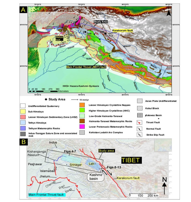
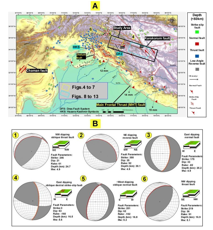
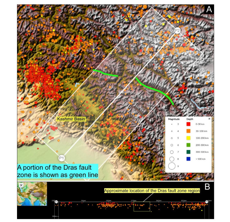
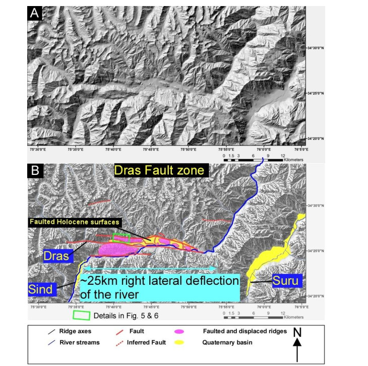
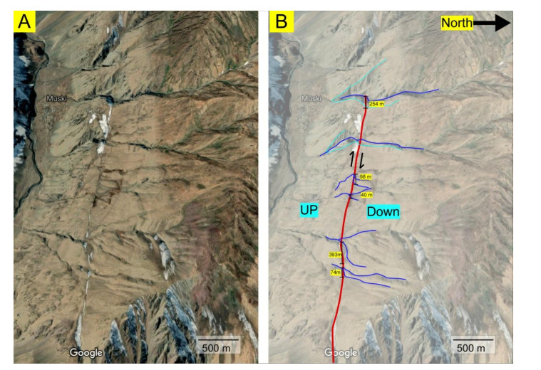
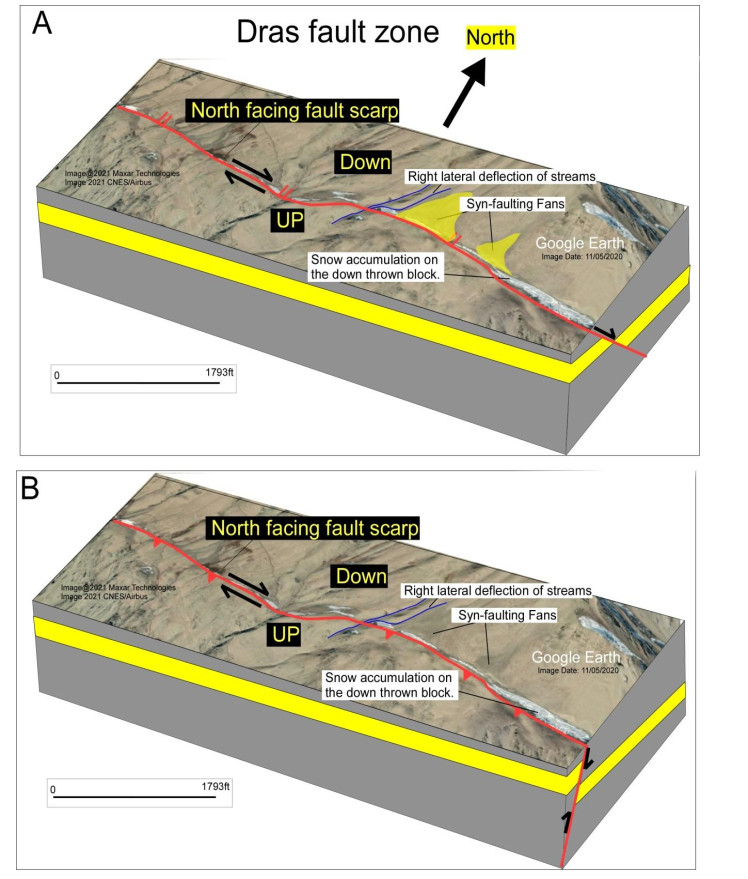
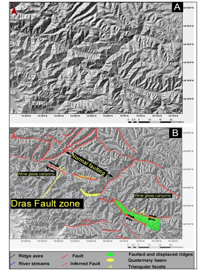
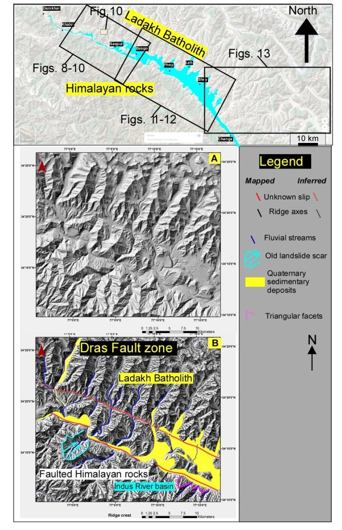
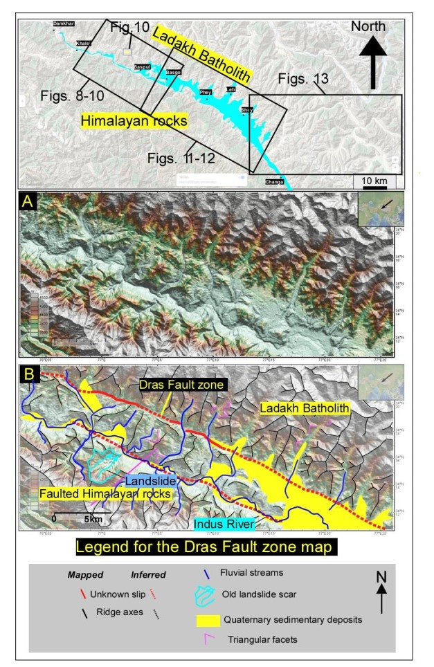
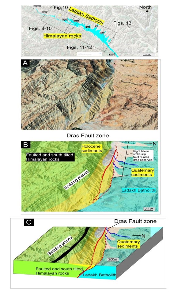
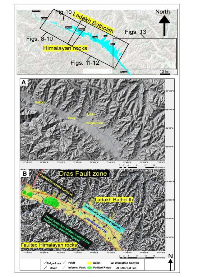
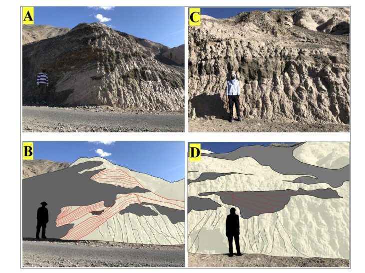
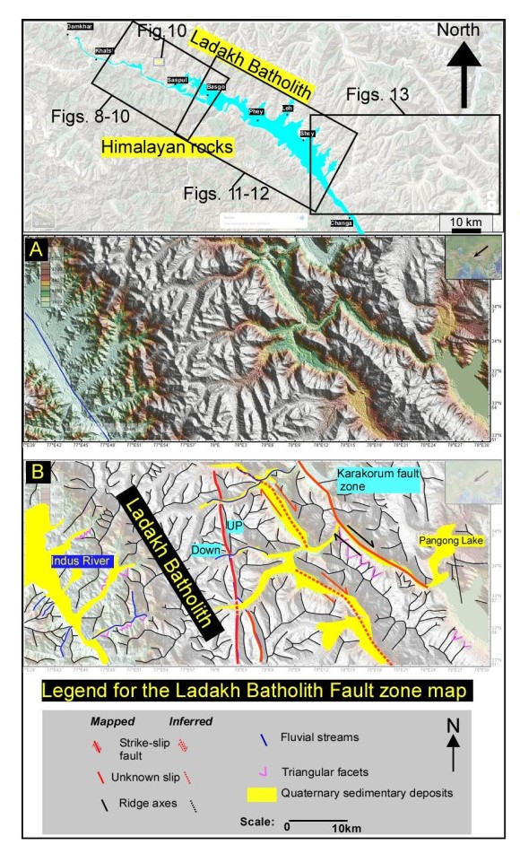
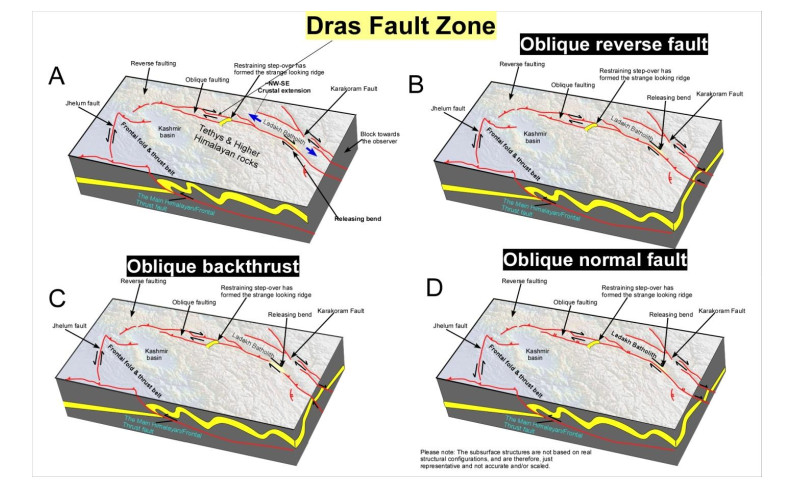
Our recent mapping of the Dras fault zone in the NW Himalaya has answered one of the most anticipated searches in recent times where strike-slip faulting was expected from the geodetic studies. Therefore, the discovery of the fault is a leap towards the understanding of the causes of active faulting in the region, and how the plate tectonic convergence between India and Eurasia is compensated in the interior portions of the Himalayan collision zone, and what does that imply about the overall convergence budget and the associated earthquake hazards. The present work is an extended version of our previous studies on the mapping of the Dras fault zone, and we show details that were either not available or briefly touched. We have used the 30 m shuttle radar topography to map the tectonic geomorphological features that includes the fault scarps, deflected drainage, triangular facets, ridge crests, faulted Quaternary landforms and so on. The results show that oblique strike-slip faulting is active in the suture zone, which suggests that the active crustal deformation is actively compensated in the interior portions of the orogen, and it is not just restricted to the frontal portions. The Dras fault is a major fault that we have interpreted either as a south dipping oblique backthrust or an oblique north dipping normal fault. The fieldwork was conducted in Leh, but it did not reveal any evidence for active faulting, and the fieldwork in the Dras region was not possible because of the politically sensitive nature of border regions where fieldwork is always an uphill task.
Citation: AA Shah, A Rajasekharan, N Batmanathan, Zainul Farhan, Qibah Reduan, JN Malik. Detailed tectonic geomorphology of the Dras fault zone, NW Himalaya[J]. AIMS Geosciences, 2021, 7(3): 390-414. doi: 10.3934/geosci.2021023
Our recent mapping of the Dras fault zone in the NW Himalaya has answered one of the most anticipated searches in recent times where strike-slip faulting was expected from the geodetic studies. Therefore, the discovery of the fault is a leap towards the understanding of the causes of active faulting in the region, and how the plate tectonic convergence between India and Eurasia is compensated in the interior portions of the Himalayan collision zone, and what does that imply about the overall convergence budget and the associated earthquake hazards. The present work is an extended version of our previous studies on the mapping of the Dras fault zone, and we show details that were either not available or briefly touched. We have used the 30 m shuttle radar topography to map the tectonic geomorphological features that includes the fault scarps, deflected drainage, triangular facets, ridge crests, faulted Quaternary landforms and so on. The results show that oblique strike-slip faulting is active in the suture zone, which suggests that the active crustal deformation is actively compensated in the interior portions of the orogen, and it is not just restricted to the frontal portions. The Dras fault is a major fault that we have interpreted either as a south dipping oblique backthrust or an oblique north dipping normal fault. The fieldwork was conducted in Leh, but it did not reveal any evidence for active faulting, and the fieldwork in the Dras region was not possible because of the politically sensitive nature of border regions where fieldwork is always an uphill task.

| [1] | Shah AA, Addly AABM, Samat MIBA (2018) Geomorphic Mapping Reveals NW-SE Extension in NW Himalaya. Arab J Geosci 385-389. |
| [2] |
Baker DM, Robert J, Robert S, et al. (1988) Development of the Himalayan frontal thrust zone: Salt Range, Pakistan. Geology 16: 3-7. doi: 10.1130/0091-7613(1988)016<0003:DOTHFT>2.3.CO;2

|
| [3] | Yeats RS, Nakata T, Farah A, et al. (1992) The Himalayan frontal fault system. Ann Tecton 6: 85-98. |
| [4] |
Wesnousky SG, Kumar S, Mohindra R, et al. (1999) Uplift and convergence along the Himalayan Frontal Thrust of India. Tectonics 18: 967-976. doi: 10.1029/1999TC900026
|
| [5] |
Malik JN, Sahoo AK, Shah AA (2010) Paleoseismic evidence from trench investigation along Hajipur fault, Himalayan Frontal Thrust, NW Himalaya: implications of the faulting pattern on landscape evolution and seismic hazard. J Struct Geol 32: 350-361. doi: 10.1016/j.jsg.2010.01.005
|
| [6] |
Wesnousky SG, Kumahara Y, Chamlagain D, et al. (2017) Geological observations on large earthquakes along the Himalayan frontal fault near Kathmandu, Nepal. Earth Planet Sci Lett 457: 366-375. doi: 10.1016/j.epsl.2016.10.006
|
| [7] |
Coudurier-Curveur A, Tapponnier P, Okal E, et al. (2020) A composite rupture model for the great 1950 Assam earthquake across the cusp of the East Himalayan Syntaxis. Earth Planet Sci Lett 531: 115928. doi: 10.1016/j.epsl.2019.115928
|
| [8] |
Cloos M (1993) Lithospheric buoyancy and collisional orogenesis: Subduction of oceanic plateaus, continental margins, island arcs, spreading ridges, and seamounts. Geol Soc Am Bull 105: 715-737. doi: 10.1130/0016-7606(1993)105<0715:LBACOS>2.3.CO;2
|
| [9] |
Tapponnier P, Molnar P (1977) Active faulting and tectonics in China. J Geophys Res 82: 2905-2930. doi: 10.1029/JB082i020p02905
|
| [10] | Keller EA (1986) Investigation of active tectonics: use of surficial earth processes. Tectonics 1: 136-147. |
| [11] | Malik JN, Nakata T (2003) Active faults and related late Quaternary deformation along the northwestern Himalayan frontal zone, India. Ann Geophys 46: 917-936. |
| [12] |
Shah AA (2013) Earthquake geology of Kashmir Basin and its implications for future large earthquakes. Int J Earth Sci 102: 1957-1966. doi: 10.1007/s00531-013-0874-8
|
| [13] | Shah AA, Sahari S, Navakanesh B, et al. (2021) Tectonic geomorphology of the Jhelum fault zone and its contiguous regions in western Himalaya. Bull Geol Soc Mal 73. |
| [14] |
Zhao LS, Xie J (1993) Lateral variations in compressional velocities beneath the Tibetan Plateau from Pn travel time tomography. Geophys J Int 115: 1070-1084. doi: 10.1111/j.1365-246X.1993.tb01510.x
|
| [15] |
Yin A (2000) Mode of Cenozoic east‐west extension in Tibet suggesting a common origin of rifts in Asia during the Indo‐Asian collision. J Geophys Res 105: 21745-21759. doi: 10.1029/2000JB900168
|
| [16] |
Stevens VL, Avouac JP (2015) Interseismic coupling on the main Himalayan thrust. Geophys Res Lett 42: 5828-5837. doi: 10.1002/2015GL064845
|
| [17] |
Shah AA (2015) Kashmir basin fault and its tectonic significance in NW Himalaya, Jammu and Kashmir, India. Int J Earth Sci 104: 1901-1906. doi: 10.1007/s00531-015-1183-1
|
| [18] | Sahoo S, Malik JN (2017) Active fault topography along Kangra valley fault in the epicentral zone of 1905 Mw7. 8 earthquake NW Himalaya, India. Quat Int 462: 90-108. |
| [19] |
Burg JP, Bouilhol P (2018) Timeline of the South-Tibet—Himalayan belt: the geochronological record of subduction, collision, and underthrusting from zircon and monazite U-Pb ages. Can J Earth Sci 56: 1318-1332 doi: 10.1139/cjes-2018-0174
|
| [20] |
Shah AA, Abd MN, Aliudin NAB, et al. (2020) Formation, Rotation, and Present-Day Configuration of Kashmir and Peshawar Basins in NW Himalaya. Front Earth Sci 8: 569771. doi: 10.3389/feart.2020.569771
|
| [21] |
Yin A, Harrison TM (2000) Geologic Evolution of the Himalayan-Tibetan Orogen. Annu Rev Earth Planet Sci 28: 211-280. doi: 10.1146/annurev.earth.28.1.211
|
| [22] |
Murphy MA, Yin A (2003) Structural evolution and sequence of thrusting in the Tethyan fold-thrust belt and Indus-Yalu suture zone, southwest Tibet. GSA Bull 115: 21-34. doi: 10.1130/0016-7606(2003)115<0021:SEASOT>2.0.CO;2
|
| [23] |
Sinclair HD, Jaffey N (2001) Sedimentology of the Indus group, Ladakh, northern India: Implications for the timing of initiation of the palaeo‐Indus River. J Geol Soc 158: 151-162 doi: 10.1144/jgs.158.1.151
|
| [24] |
Garzanti E, Haver TV (1988) The Indus clastics: Fore‐arc basin sedimentation in the Ladakh Himalaya (India). Sediment Geol 59: 237-249. doi: 10.1016/0037-0738(88)90078-4
|
| [25] |
Searle MP, Pickering KT, Cooper DJW (1990) Restoration and evolution of the intermontane Indus molasse basin, Ladakh Himalaya, India. Tectonophysics 174: 301-314. doi: 10.1016/0040-1951(90)90327-5
|
| [26] |
Searle MP (1986) Structural evolution and sequence of thrusting in the High Himalayan, Tibetan—Tethys and Indus suture zones of Zanskar and Ladakh, Western Himalaya. J Struct Geol 8: 923-936. doi: 10.1016/0191-8141(86)90037-4
|
| [27] |
Qayyum M, Lawrence RD, Niem AR (1997) Discovery of the palaeo-Indus delta-fan complex. J Geol Soc 154: 753-756. doi: 10.1144/gsjgs.154.5.0753
|
| [28] | Nakata T (1989) Active faults of the Himalayas of India and Nepal. Spec Pap Geol Soc Am 232: 243-264. |
| [29] | Sahoo S, Malik JN (2017) Active fault topography along Kangra valley fault in the epicentral zone of 1905 Mw7. 8 earthquake NW Himalaya, India. Quat Int 462: 90-108. |
| [30] | Shah AA, Syaakiirroh Sahari, Navakanesh B, et al. (2022) Tectonic geomorphology of the Jhelum fault zone and its contiguous regions in western Himalaya. Bull Geol Soc Malay 73. |
| [31] |
Shah AA, Navakanesh B (2020) Active tectonics and active faults: Why these terms still lack consensus on definitions. Bull Geol Soc Malay 70: 125-132. doi: 10.7186/bgsm70202010
|
| [32] | DiPietro JA, Pogue KR (2004) Tectonostratigraphic subdivisions of the Himalaya: A view from the west. Tectonics 23. |
| [33] | Jouanne F, Munawar N, Mugnier JL, et al. (2020) Seismic coupling quantified on inferred décollements beneath the western syntaxis of the Himalaya. Tectonics 39. |
| [34] | Shah AA, Rajasekharan A, Batmanathan N, et al. (2021) Dras Fault: a major active fault in Kashmir Himalaya. Bull N Z Soc Earthq Eng 30. |
| [35] | Sangode SJ, Phadtare NR, Meshram DC, et al. (2011) A record of lake outburst in the Indus valley of Ladakh Himalaya, India. Curr Sci 100: 1712-1718. |
| [36] |
Gansser A (1980) The significance of the Himalayan suture zone. Tectonophysics 62: 37-52. doi: 10.1016/0040-1951(80)90134-1
|
| [37] |
Searle MP (1983) Stratigraphy, structure and evolution of the Tibetan-Tethys zone in Zanskar and the Indus suture zone in the Ladakh Himalaya. Earth Environ Sci Trans R Soc Edinb 73: 205-219. doi: 10.1017/S0263593300009688
|
| [38] | Ahmad SA, Sahari S, Qadir A, et al. (2020) A critical review of field relationships and gravitational origin of active normal faults in the Kashmir basin, NW Himalaya. J Asian Earth Sci X 100042. |
| [39] |
Schiffman C, Bali BS, Szeliga W, et al. (2013) Seismic slip deficit in the Kashmir Himalaya from GPS observations. Geophys Res Lett 40: 5642-5645. doi: 10.1002/2013GL057700
|
| [40] |
Kundu B, Yadav RK, Bali BS, et al. (2014) Oblique convergence and slip partitioning in the NW Himalaya: Implications from GPS measurements. Tectonics 33: 2013-2024. doi: 10.1002/2014TC003633
|
| [41] |
Bilham R (2019) Himalayan earthquakes: a review of historical seismicity and early 21st century slip potential. Geol Soc Spec Publ 483: 423-482. doi: 10.1144/SP483.16
|
| [42] | Omar Pengiran DNA, Shah AA, Abd MN (2020) Active transtensional structures mapped in the west of Karakoram fault (KF), Kashmir Himalayas. 5th International Young Earth Scientists (YES) Congress "Rocking Earth's Future". |
| [43] |
Koukouvelas IK, Zygouri V, Papadopoulos GA, et al. (2017) Holocene record of slip-predictable earthquakes on the Kenchreai Fault, Gulf of Corinth, Greece. J Struct Geol 94: 258-274. doi: 10.1016/j.jsg.2016.12.001
|
| [44] |
Koukouvelas IK, Zygouri V, Nikolakopoulos K, et al. (2018) Treatise on the tectonic geomorphology of active faults: The significance of using a universal digital elevation model. J Struct Geol 116: 241-252. doi: 10.1016/j.jsg.2018.06.007
|
Figures(14)

AA Shah, A Rajasekharan, N Batmanathan, Zainul Farhan, Qibah Reduan, JN Malik. Detailed tectonic geomorphology of the Dras fault zone, NW Himalaya[J]. AIMS Geosciences, 2021, 7(3): 390-414. doi: 10.3934/geosci.2021023


 DownLoad: