


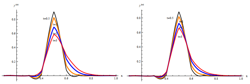
Figure 1.
The time evolution of the approximate solutions of the classical case β=1, left, and for the non classical case β=0.75, right.
The Feller exponential population growth is the continuous analogues of the classical branching process with fixed number of individuals. In this paper, I begin by proving that the discrete birth-death process, M/M/1 queue, could be mathematically modelled by the same Feller exponential growth equation via the Kolmogorov forward equation. This equation mathematically formulates the classical Markov chain process. The non-classical linear birth-death growth equation is studied by extending the first-order time derivative by the Caputo time fractional operator, to study the effect of the memory on this stochastic process. The approximate solutions of the models are numerically studied by implementing the finite difference method and the fourth order compact finite difference method. The stability of the difference schemes are studied by using the Matrix method. The time evolution of these approximate solutions are compared for different values of the time fractional orders. The approximate solutions corresponding to different values of the birth and death rates are also compared.
Citation: E. A. Abdel-Rehim. The time evolution of the large exponential and power population growth and their relation to the discrete linear birth-death process[J]. Electronic Research Archive, 2022, 30(7): 2487-2509. doi: 10.3934/era.2022127
| [1] | Wenjing An, Xingdong Zhang . An implicit fully discrete compact finite difference scheme for time fractional diffusion-wave equation. Electronic Research Archive, 2024, 32(1): 354-369. doi: 10.3934/era.2024017 |
| [2] | Chang Hou, Hu Chen . Stability and pointwise-in-time convergence analysis of a finite difference scheme for a 2D nonlinear multi-term subdiffusion equation. Electronic Research Archive, 2025, 33(3): 1476-1489. doi: 10.3934/era.2025069 |
| [3] | Jun Pan, Yuelong Tang . Two-grid $ H^1 $-Galerkin mixed finite elements combined with $ L1 $ scheme for nonlinear time fractional parabolic equations. Electronic Research Archive, 2023, 31(12): 7207-7223. doi: 10.3934/era.2023365 |
| [4] | Mingfa Fei, Wenhao Li, Yulian Yi . Numerical analysis of a fourth-order linearized difference method for nonlinear time-space fractional Ginzburg-Landau equation. Electronic Research Archive, 2022, 30(10): 3635-3659. doi: 10.3934/era.2022186 |
| [5] | Li Tian, Ziqiang Wang, Junying Cao . A high-order numerical scheme for right Caputo fractional differential equations with uniform accuracy. Electronic Research Archive, 2022, 30(10): 3825-3854. doi: 10.3934/era.2022195 |
| [6] | Yunxia Niu, Chaoran Qi, Yao Zhang, Wahidullah Niazi . Numerical analysis and simulation of the compact difference scheme for the pseudo-parabolic Burgers' equation. Electronic Research Archive, 2025, 33(3): 1763-1791. doi: 10.3934/era.2025080 |
| [7] | Ming-Kai Wang, Cheng Wang, Jun-Feng Yin . A class of fourth-order Padé schemes for fractional exotic options pricing model. Electronic Research Archive, 2022, 30(3): 874-897. doi: 10.3934/era.2022046 |
| [8] | Leilei Wei, Xiaojing Wei, Bo Tang . Numerical analysis of variable-order fractional KdV-Burgers-Kuramoto equation. Electronic Research Archive, 2022, 30(4): 1263-1281. doi: 10.3934/era.2022066 |
| [9] | Guoliang Zhang, Shaoqin Zheng, Tao Xiong . A conservative semi-Lagrangian finite difference WENO scheme based on exponential integrator for one-dimensional scalar nonlinear hyperbolic equations. Electronic Research Archive, 2021, 29(1): 1819-1839. doi: 10.3934/era.2020093 |
| [10] | Noelia Bazarra, José R. Fernández, Ramón Quintanilla . On the mixtures of MGT viscoelastic solids. Electronic Research Archive, 2022, 30(12): 4318-4340. doi: 10.3934/era.2022219 |
The Feller exponential population growth is the continuous analogues of the classical branching process with fixed number of individuals. In this paper, I begin by proving that the discrete birth-death process, M/M/1 queue, could be mathematically modelled by the same Feller exponential growth equation via the Kolmogorov forward equation. This equation mathematically formulates the classical Markov chain process. The non-classical linear birth-death growth equation is studied by extending the first-order time derivative by the Caputo time fractional operator, to study the effect of the memory on this stochastic process. The approximate solutions of the models are numerically studied by implementing the finite difference method and the fourth order compact finite difference method. The stability of the difference schemes are studied by using the Matrix method. The time evolution of these approximate solutions are compared for different values of the time fractional orders. The approximate solutions corresponding to different values of the birth and death rates are also compared.
The mathematical modelling of biological problems always gains the interest of many researchers. The birth-death process introduced by Yule [1], Feller [2] and Kendall [3], represents a natural theoretical framework of different biological studies. Such studies have various applications as population dynamics, genome evolution and etc.. In this paper, I am interested in studying the asexual reproduction of like-individual (organisms, cells, genome, etc.). Beginning by the classical branching process that describes a large population that consists initially of Ne like haploid individuals. In each succeeding generation with assuming non-overlapping, the population produces asexually like individuals with number N(t). Each one of them may give birth to 0,1,2,⋯, individuals with corresponding probabilities p0,p1,p2,⋯ such that ∑kpk=1. The individuals of any generation are independent identically distributed random (i.i.d.r.) numbers. The number of individuals in the n-th generation is denoted by a random variable (r.v.) of a Markov-Type. Kolmogorov [4] mathematically formulated this model in the form of the Fokker-Planck equation, namely
| ∂u(x,t)∂t=(b(x)u(x,t))xx−(a(x)u(x,t))x=Lfpu(x,t),0<x<∞,t≥0, | (1.1) |
where the indepenedent random variable x represents the size and u(x,t) is a probability density function being subjected to the initial condition u(x,0)=δ(x), and there is no boundary conditions imposed on it. a(x) is the expected number of individuals and b(x) is its variance. Kolmogorov assumed in his derivation of (1.1) that the only restriction imposed on the number of the population size Ne is that it is fixed at any generation.
Later, Feller [5], assumed that the density function u(x,t) is independent of on the total population size Ne and formulated his exponential growth equation as
| ∂u(x,t)∂t=γ(xu(x,t))xx−α(xu(x,t))x,0<x<∞,t≥0, | (1.2) |
where α and γ are initially assumed to be constants. This equation is called by Feller [5], the exponential population growth because its expected population size is obtained as
| M(t)=∞∫0xu(x,t)dx=Neeαt. | (1.3) |
That means M(t) is growing up exponentially. α represents the actual rate of population increase and can be written as α=1tln(M(t)Ne). The variance could be written as
| σ2=2γαM(t)Ne(M(t)Ne−1),Ne≠0,M(t)>N0. | (1.4) |
Then according to Feller, the mean and the variance are necessarily proportional to the instantaneous population size N(t). As α>0 the population average increases, as α<0 the population decreases. Feller stated that the analytic unique solution of Eq (1.2) could be written in terms of the Bessel function I1, see for more details [5]. According to Feller, the probability that the population dies out before time t is
| Δ(t)=exp(−αNeγ11−e1−αt),t>>0, | (1.5) |
and on the long run, i.e., as t→∞, the probability that there is no individual exists is given as
| Δ={e−αNeγ,α>01,α<<0. |
For more details about the difference views between the pioneers of the population genetics researchers and the modern studies, see Ewens [6]. Dutykh [7], give an approximate solution of the classical Feller's Eq (1.2) after replacing the drift term (a(x)u(x,t))x by ((ax+cu(x,t)))x. The author reformulated the equation by the so called Lagrangian or material variables, to avoid the unbounded of its variable coefficients. Masoliver [8] studied the non-stationary classical Feller process with time-varying coefficients. The author obtained the exact probability distribution and prove as Ross proved that the probability density function approaches the Gamma distribution on the long run. Recently, Giorno et al. [9] studied the time-inhomogeneous Feller-Type diffusion process in the population dynamics. The authors calculated the expectation, the moment generating function and the periodicity of the density function of the classical diffusion of the birth-death process with immigration.
The discrete birth-death process or the so called M/M/1 exponential model, represents a system in which an individual (customer) joins a system for having a specific service with rate λ and the service (leaving or death) rate is μ with λμ<1. The server is serving only one customer at each time instant. The probability of finding m (customers) at any time n at the system has the same meaning of the asexual production being studied by Fokker-Planck and is mathematically formulated by Eq (1.1).
In this paper, I am interested in proving that the discrete birth-death process, with random birth rate λ and with random death rate μ is mathematically formulated by the same Eq (1.1) as the birth and death rats are linearly growth. I am interested also in studying the approximate solution of Eq (1.1), for many cases. The first case, is to assume that the number of individuals is fixed at any generation. The second case is to assume that the number of individuals are randomly vary from a generation to generation. Finally is to add the memory effects on the diffusion process Eq (1.1) by extending the first order time derivative to the Caputo time-derivative, namely
| CDβ0tu(x,t)=γ(xu(x,t))xx−α(xu(x,t))x,0<x<∞,t≥0,0<β<1. | (1.6) |
I prefer to call this equation the time-fractional linear population growth equation. This is allowed as Eq (1.1) represents a solution of a stochastic process and u(x,t)→0,xnu(x,t)→0 as x→∞ for all n∈N0, see reference [12] for more details about the extension of partial differential equation to fractional differential equation.
For this aim, I implement two numerical methods. The first method is the finite difference method and the second is the fourth order compact finite difference method. The Grünwald-Letnikov scheme is utilized to find the the discrete scheme of the Caputo time-fractional operator. Abdel-Rehim, see for example [10,11,12], has successfully used the Grünwald-Letnikov scheme to simulate many time-fractional diffusion equations. Talib et al. [13] used another numerical method based on the operational matrices to find the numerical solutions of time-fractional differential equations. The authors used the Caputo and the Riemann-Liouville of two-parametric orthogonal shifted Jaccobi polynomials. Talib et al. [14] has recently generalized the existing operational matrix method to operational matrix of mixed partial derivative terms in Caputo sense. In this improvement, the authors used the orthogonal shifted Legendre polynomials.
It is worth to say that Polito et al.[15] studied a fractional birth-death process. The authors presented in their paper a subordination relationship connected the fractional birth-death process with the classical birth-death process. Later Polito [16] studied the generalized Yule models. Recently, Ascion et al. [17] studied some non-local diffusion-differential equations related to the birth-death processes and are appeared as discrete approximations of Pearson diffusions. The authors in these papers used the branching processes and the stochastic processes tools to discuss theoretically the fractional birth-death process.
To this aim, the paper is organized as follows. Section 1 is devoted to the introduction. Section 2 is to derive the diffusion equation of the linear birth-death discrete exponential model. Section 3, is to derive the approximate discrete solutions of the classical (Markov) and non-classical (Non-Markov) linear birth-death process by the finite difference method. Section 4, is for driving the approximate solutions by the fourth order compact finite difference method. Finally, section 5, is to present and to discuss the numerical results.
The birth death process is a stochastic process being defined as {X(t)=n,t≥0}, where its states X(0)=0,X(1)=1,X(2)=2,⋯ represent the number of customers or the number of (similar individuals) exist in the system at any time t, n∈N0. Now suppose two time instants t,t+τ with τ→0 and two non negative integers i,j that represent the number of individuals [18]. Define the continuous time Markov chain's transition probability from the state X(t) with i number of individuals to its neighbour X(t+τ) with j number of individuals as
| P(t+τ)=P{X(t+τ)=j|X(t)=i,X(t−τ)=i1,X(t−2τ)=i2,⋯,X(1)=in−1,X(0)=in}=P{X(t+τ)=j|X(t)=i}, | (2.1) |
or in other words, the process in the sate X(t+τ), depends only in the previous state X(t), and not on all the previous states, i.e., the the process has no memory. The Bays formula for the continuous time Markov chain
| P(t+τ)=∑k=0=P(X(t+τ|X(t)=k)P(X(t)=k). |
The Kolmogorov's forward equation of the discrete Markov chain reads
| Pij(t+τ)=∑k=0Pik(τ)Pkj(t). |
Subtract Pij from both sides, where for small τ, one can set Pij(t)=(1−Pii(τ))Pij(t). So far, one gets
| Pij(t+τ)−Pij(t)=∑k≠iPik(τ)Pkj(t)−(1−Pii(τ))Pij(t), |
where Pii≠0,∀i≥0, i.e., there is no absorbing states and ∑jPij=1. If Pii(τ) is the probability that the process is in state i and will stay in i at the time τ, the 1−Pii is the probability that the process is no longer in state i. Now divide both sides by τ and take the limit as τ→0, to get
| ∂Pij(t)∂t=∑k≠iCiPkj(t)−DiPij(t), | (2.2) |
where Ci=limτ→0Pikτ, and Di=limτ→01−Piiτ are constants. For the birth-death process with birth rate λi and death rate μi, see [18], and for j=0, i.e. the system is empty, one has
| ∂Pij(t)∂t=μ1Pi1(t)−λ0Pi0(t). | (2.3) |
This equation represents also the exponential queueing model M/M/1 in which there is only one customer in the system and is being served and no one joins the queue. The only restriction for the the queueing system is that λμ<1, to ensure that all the customers will be served. For j≥1, one has
| ∂Pij(t)∂t=λj−1Pij−1(t)−(λj+μj)Pij(t)+μj+1Pij+1(t), | (2.4) |
λj,(1−(λj+μj)),μj are the possible transition probabilities from the state Xj at the time instant tn to the sates Xj+1,Xj,Xj−1, respectively, at the time instant tn+1, where Xj=jh. This equation represents the M/M/1 queue in which customers arrive according to Poisson process with arrival rate λj and the customer is served with rate μj and the time of serving is an exponential random variable.
This equation represents also the first order time derivative of the transition probability Pij at any time instant tn, n≥0. For simplicity write Pij=Pj, ∀i, and the same for the birth and death rates. The solution of Eq (2.4) represents the probability of finding j individuals at the system at any time t. Now suppose the number of customers in the system, the number of individuals exists at the colony, or the queueing system, are very large. or in other words j→∞, and for mathematical convenience replace j by x. Then one can write λj−1Pj−1=λ(x−h)P(x−h), with h→0, (λj+μj)Pj=(λ(x)+μ(x))P(x), and μj+1Pj+1=μ(x+h)P(x+h), where h is the space instant and h→0. Now, Eq (2.4), could be rewritten as
| ∂P(x,t)∂t=λ(x−h)P(x−h)+(λ(x)+μ(x))P(x)+μ(x+h)P(x+h), | (2.5) |
and now the Taylor's expansion can be used to expand the terms λ(x−h)P(x−h) and μ(x+h)P(x+h), to get
| ∂P(x,t)∂t=h22∂2∂x2(λ(x)p(x)+μ(x)p(x))−h∂∂x(λ(x)p(x)−μ(x)p(x))+O(h3). | (2.6) |
The functions λ(x) and μ(x) could be any smooth convergent functions. For linear birth-death process, one has to choose λ(x)=λx and μ(x)=μx, and henceforth Eq (2.6) is rewritten as
| ∂P(x,t)∂t(x,t)=h22(λ+μ)∂2∂x2(xp(x,t))−h(λ−μ)∂∂x(xp(x)). | (2.7) |
Let R be the number of x steps and put h=1/R, and define the coefficients
| γ=12R2(λ+μ),α=(λ−μ)R,R∈N, | (2.8) |
then Eq (2.7), with Eq (2.8) is identical with Eq (1.2), and is called the linear birth-death process. The linear birth-death process is a stochastic exponential model with random birth rate, rate of arrivals, λ∈(0,1) and random death rate μ∈(0,1), rate of departure or rate of service. The right hand side of Eq (2.7) is a special the form of the Fokker-Planck operator Lfp, see [12]. So far I prefer to write the linear birth-death process as
| ∂P(x,t)∂t(x,t)=LfpP(x,t). | (2.9) |
The waiting time between any two successive arrivals (birth) and departures (death) are exponentially distributed as e−λt and e−μt, respectively. The values of λ and μ could be fixed random number at all the next generations and could be computed as exponential random variables at each generation. The expected population size Eq (1.3) of Eq (2.7) is obtained as
| M(t)=∞∫0xu(x,t)dx=Neexp(t(λ−μ)R). | (2.10) |
As λ>μ, the population increases and as λ<μ, the population decreases. In the next section, I am going to derive the discrete approximate solution of Eq (1.2), with its α and γ are calculated by Eq (2.8), by the explicit finite difference method (fdm).
I am beginning the discussion of the approximate solution by the common rules of the explicit fdm as the basic of all the numerical methods. Define the nth-time step as
| tn=nτ,τ>0,n∈N0. | (3.1) |
Introduce the clump y(n) as
| y(n)={y(n)1,y(n)2,⋯,y(n)R−2,y(n)R−1}T, | (3.2) |
where y(n)=y(tn) represents the discrete probability column vector to find m individual at the generation tn or at the time instant tn. To solve the partial differential Eq (1.2) and its equivalent Eq (2.7), the initial value y(0) has to satisfy R−1∑j=1y(0)j=1, ∀n∈N0. The proper choice is u(x,0)=δ(x), hence fourth
| y(0)={0⋯,1,⋯,0}T. | (3.3) |
The discrete scheme of Eq (2.7), reads
| yn+1j−ynjτ=γh2[h(j+1)ynj+1−2hynj+h(j−1)ynj−1]−α2h[(j+1)hynj+1−(j−1)hynj−1]+O(h2+τ), | (3.4) |
where n≥0. Define the scaling relation η=τh2, and solve for y(n+1)j, to get
| y(n+1)j=η(j−1)(γR+α2R2)y(n)j−1+(1−2jηγR)y(n)j+η(j+1)(γR−α2R2)y(n)j+1, | (3.5) |
where n≥0 and y(n+1)j represents the discrete probability density function of finding the system at the time instant tn+1 with m individuals. Summing the coefficients of the y(n)j−1,y(n)j,y(n)j+1, one can easily find R−1∑j=1y(n+1)j=1. The difference scheme (3.5) is stable and convergent if the scaling relation η satisfies the following condition
| 0<η≤R2jγ,1≤j≤R−1, | (3.6) |
and for the suitable choice as j=R2, one gets η≤1γ. The difference scheme (3.5), could be written in a matrix form as
| y(n+1)=PT.y(n),n≥0, | (3.7) |
where the matrix P=Pij is R−1×R−1 and is defined as
| Pij={P(1)ij=η(j−1)(γR+α2R2),i=j−1,j=1,⋯,R−1P(2)ij=(1−2jηγR),i=j,j=1,⋯,R−1P(3)ij=η(j+1)(γR−α2R2),i=j+1,j=1,⋯,R−1. | (3.8) |
For proving the stability of this approximate solution, define the two column vectors Λ and 0, with length R−1 as
| Λ={1,1,⋯,1}T,0={0,0,⋯,0}T. |
The matrix P is stable if it satisfies the two equal conditions
| ||PT||∞=max{||PT.ΛΛ||,||Λ≠0||} | (3.9) |
or
| ||PT||∞=max1≤i≤R−1R−1∑j=1Pij. | (3.10) |
Since P is a stochastic matrix, and PT.Λ=Λ, i.e., the sum over all its rows is 1. The matrix P satisfies the both stability conditions. The greatest eigenvalue of P is 1, then its spectral radius being defined as
| ρ(PT)=max1≤i≤Rζi, | (3.11) |
where {ζi} is the set of the eigenvalues of PT. Then for this case ρ(PT)≤||PT||∞=1, see [19] for more details about the stability of the explicit difference methods of the diffusion convection equations. Now for the purpose of computation, it is better to take the transpose of Eq (3.7) and rewrite it as
| z(n+1)=z(n).(I+η.H1),n≥0, | (3.12) |
where z(n)=(y(n))T, I is the unit matrix. H1T is the matrix that satisfies H1T.Λ=0, i.e., the sum over all its rows is zero, and being defined as
| H1ij={H1(1)ij=η(j−1)(γR+α2R2),i=j−1,j=1,⋯,R−1H1(2)ij=−2jηγR,i=j,j=1,⋯,R−1H1(3)ij=η(j+1)(γR−α2R2),i=j+1,j=1,⋯,R−1. | (3.13) |
The transition probabilities at Eq (3.5), constitute a Markov chain. Therefore, the waiting time between every two random events, arrivals of a new individual, is ≈e−t, i.e., is exponentially distributed. That means this stochastic process at the time instant tn+1, depends only on the time instant tn, and neither nor all its previous history. In Reality, this is not correct and the history of the process has to be considered. In other words the number of individuals at the time instants tn−1, tn−2, ⋯,t0, should be known.
Now, to find the approximate solution of the time-fractional linear growth defined in Eq (1.6). The Caputo time fractional operator of order β is defined for a smooth function f(t) as
| CDβ0tf(t)={1Γ(n−β){t∫0f(n)(τ)Kβ(t−τ)dτ}forn−1<β<n,dndtnf(t)forβ=n, | (3.14) |
where
| Kβ(t−τ)=(t−τ)β+1−nΓ(n−β). |
The kernel Kβ(t−τ) represents the memory function, and it reflects the memory effects of many physical, biological and etc. processes, see [22] and [23].
Before going on our descretization of the Caputo fractional operator, I give a quick review about the advantages of using this operator on modelling the read–world problems. to do so, recall the definition the Riemann-Liouville fractional integral operator, denoted by Jβ, as
| Jβf(t)=1Γ(β)t∫0f(τ)(t−τ)(1−β)dτ,t>0,β>0. | (3.15) |
For completeness, one sets J0f(t)=f(t). This means J0 is an identity operator. The Riemann-Liouville fractional derivative operator, for a sufficiently smooth function f(t) given in an interval [0,∞), is defined as (see for example:[25] and [24])
| (Dβf)(t):={1Γ(m−β)dmdtm∫t0f(τ)(t−τ)β+1−mdτ,m−1<β<m,dmdtmf(t),m=β, | (3.16) |
and
| Dβf(t)=D1J1−βf(t). |
From the definitions (3.15) and (3.16), we can define the Riemann-Liouville fractional derivative Dβ as the left inverse of Jβ, β≥0. Therefore some authors prefer to write the Riemann-Liouville fractional integral operator Jβ as D−β (e.g. [25,26,27]). For completeness, we have D0=I. One can deduce from the two definitions (3.14) and (3.16) that both the operators are non local but both have different kernels. The definition of Caputo is restrictive than Eq (3.16) because it requires that f(m)(t) exists. therefore, Caputo is more convenience for the mathematical manipulations. For completeness, we have D0=I.
The Riemann-Liouville fractional derivative of the power function tμ, gives
| Dβtμ=Γ(μ+1)Γ(μ+1−β)tμ−β,β≥0. |
This means the Riemann-Liouville fractional derivative of a non-zero constant is different from zero. In fact
| Dβ1=Dβt0=Γ(1)Γ(1−β)t−β,0<β<1. |
This is the main disadvantage of this operator. But CDβ0tf(t)=I as β=0. The Caputo operator with the Riemann-Liouville satisfies the relation
| CDβ0tf(t)=Jm−βDmf(t),m−1<β≤m, |
Caputo can also be defined through its image in the Laplace transform domain, which is
| L{Dβ∗f(t);s}=sβ˜f(s)−sβ−1f(0)−ˊf(0)sβ−2−⋯−f(m−1)(0)sβ−m,s>0. |
The Caputo fractional derivative of order, in the special case 0<β≤1 satisfies also
| CDβ0tf(t)=J1−βDf(t)=Dβ∗(f(t)−f(0+)), | (3.17) |
and
| Dβ(f(t)−f(0))=DJ1−β(f(t)−f(0))=Dβf(t)−f(0)Γ(1−β)t−β, | (3.18) |
we can deduce that
| CDβ0tf(t)=Dβ(f(t)−f(0)),0<β≤1, | (3.19) |
This is the second difference between the Caputo and the Riemann Liouville derivatis. In other words, the Caputo depends on the initial condition of the function f(t). Recently Diethelm [29] stated in his book "The Main Disadvantage of the Riemann-Liouville Fractional Derivative is that it Fails to Model the Real World Phenomena of Fractional Differential Equation.".
For discretizing the Caputo time-fractional derivative, I utilize the Grünwald- Letnikov scheme being reads
| CDβ0ty(n+1)j=n+1∑k=0(−1)k(βk)y(n+1−k)j−y(0)jτβ,0<β≤1. | (3.20) |
where
| CD0t1y(n+1)j=1τ(y(n+1)j−y(n)j). |
To find the average number of individuals of this memory-dependent process M(t) defined in Eq (1.3), it is important to write Eq (1.6) in terms of the Fokker-Planck operator Lfp and the Riemann-Liouville fractional derivative operator D0tβ, as
| CDβ0tu(x,t)=D0tβ[u(x,t)−u(x,0)]=Lfpu(x,t), | (3.21) |
See reference [24]. This equation can also be written as
| u(x,t)−u(x,0)=D0t−β(Lfpu(x,t)), | (3.22) |
where D0t−β=Jβ, is the Riemann-Liouville fractional. Now multiply both sides of Eq (3.22) by x and integrate over x∈[0,∞), with regarding the initial condition u(x,0)=δ(x), and by using the natural properties of u(x,t) as probability density function, namely u(x,t)→0, x∂u∂x→0 and x∂2u∂x2→0 as x→∞, to get
| CDβ0tM(t)=−αM(t). | (3.23) |
This equation has the solution
| M(t)=Eβ(−αtβ), | (3.24) |
which is a special form of the so called Mittag-Leffler function. In the special case as β=1, it is identical to the exponential function e−αt, for its simulation see reference [12]. That means the special case as β gives the same exponential average of individuals defined in Eq (2.10) but as 0<β<1, the average M(t) exhibits proportionally as the power function αt−(β+1). Abdel-Rehim [38] has recently simulated the asymptotic behaviour of the Mittag-Leffler function and compared the results with the exponential function e−t and Hypergeometric1F1[1+n,2+n,−t] function, for different values of t, β and n. Now the discrete scheme of the time-fractional population growth Eq (1.6) reads
| y(n+1)j−βy(n)j−n+1∑k=2(−1)k(βk)y(n+1−k)j−n+1∑k=0(−1)k(βk)y(0)j=γτβh2[h(j+1)ynj+1−2hynj+h(j−1)ynj−1]−ατβ2h[(j+1)hynj+1−(j−1)hynj−1], | (3.25) |
where its error is of order O(h2+τβ). For convenience, recall the following coefficients
| bn=n+1∑k=0(−1)k(βk),n=0,1,2,… |
| ck=(−1)k+1(βk),k=1,2,…, |
which are introduced by Gorenflo et al. [28]. These coefficients satisfy that b0=c1=β, all ck≥0, bn≥0, ∞∑k=1ck=1, and finally satisfy the relation
| bn+n∑k=1ck=1. | (3.26) |
Assuming the new scaling relation as η=τβh2, rearranging the terms of Eq (3.25) and solving for y(n+1)j, to get
| y(n+1)j=n+1∑k=0bny(0)j+n+1∑k=2cky(n+1−k)j+(β−2jηγR)y(n)j+η(j−1)(γR+α2R2)y(n)j−1+η(j+1)(γR−α2R2)y(n)j+1, | (3.27) |
where n≥1. For computing y(n+1)j, the values of y(n)j, y(n−1)j, y(n−2)j, ⋯,y(0)j, should be known. That means the diffusion process for n≥1, depends on all the history, the process has a memory. That what is called the Non-Markov process. The difference scheme (3.27), is convergent if the coefficient of y(n)j, is positive and that requires that the scaling relation of this non-classical case should satisfy
| 0<η≤βR2jγ, | (3.28) |
and again by choosing j=R/2, one gets a suitable condition for the scaling relation η. The difference scheme (3.27) could be written in the matrix form as
| z(n+1)=n+1∑k=0bnz(0)j+n+1∑k=2ckz(n+1−k)j+z(n).(βI+η.H1),n≥1. | (3.29) |
Again the difference scheme (3.27) is stable as the matrix (βI+η.H1)T.Λ=βΛ, then ||(βI+η.H1)T||∞=β with 0<β<1. That satisfies the stability condition (3.9), and hence forth the second condition (3.10) is satisfied. The maximum eigenvalue of the matrix (βI+η.H1)T is β<1, therefore the spectral radius being defined as of this difference scheme is ρ(βI+η.H1)T<1. Then this difference scheme is stable and the scaling relation condition (3.28) ensures its convergence. Abdel-Rehim [20] proved that the waiting time between every two arrivals (events) on the time-fractional diffusion processes is the Mittag-Leffler function, see also [21] and the references therein for more details about the job of the Mittag-Leffler function on the continuous time random walk.
For n=0, this is the first state after the initial state. By returning back to Eq (3.25), we find that y(1) represents the probability of finding the system at the state X(1). Therefore, the approximate solution as n=0, is computed according to Eq (3.12) as
| z(1)=z(0).(I+η.H1),n≥0, | (3.30) |
and in this case, the transitions could be described as a Markov chain. In the following section, I use the fourth order compact finite difference method (focfd) to derive the stable difference scheme of studied models to be compared with the results obtained by fdm.
The finite difference method used in the above section has many advantages such as: it is computationally efficiency, requires simple code structures and it maintain the mass conservation. Its only disadvantage is that it is irregular geometric matching. To interpret this sentence suppose that f(x) is a smooth continuous function and its derivative fx=df(x)dx exists. define the truncation error by O. Define also xi=ih, xi+1=x+h, and xi−1=x−h. Then one deduce
| fx(xi)=f(xi)−f(xi−1)h,O(h) |
and
| fx(xi)=f(xi+1)−f(xi−1)2h,O(h2). |
In general
| fx(xi)≈n∑j=−nαjf(xi+j),O(hn). |
That means to obtain a truncation error of order O(hn), one needs to use 2n+1 values of f(x) to approximate fx(xi). Therefore, the fdm is inconvenience for solving the partial differential equations with variable coefficients near the boundaries.
The focfd did overcome this trouble by adding more nodes with few grid points smaller mesh sizes, in order to obtain a higher order of truncation error.
The focfd has been proved and implemented by many authors. It has been proved that the obtained approximate solution is approximately consistent with the exact solution, especially of the advection convection equations, than by using the common fdm rules.
Turkel and Singer [30], introduced limited grid sizes to make the high-order compact finite difference schemes produce more accurate solutions. Later [33], the focfd is improved by eliminating the convection term to make it more easier to implement the central difference schemes to solve convection-diffusion equations efficiently. For more details about the advantages and the disadvantages of the compact finite difference methods, see [31,32,34,35,36]. One can deduce from these references that the main advantage of the focfd is the high accuracy.
It is known that the first δxy(n)j and the second δ2xy(n)j classical spatial discrete central finite difference operators are defined as
| δxy(n)j=y(n)j+1−y(n)j−12h,δ2xy(n)j=y(n)j+1−2y(n)j+y(n)j−1h2, | (4.1) |
where the clump y(n), for this method, is defined as
| y(n)={y(n)2,y(n)2,⋯,y(n)R−2,y(n)R−2}T. | (4.2) |
To implement the focfd one has to use 1st derivative operator that is defined as, see references [33,34],
| (∂y∂x)(n)j=δxy(n)j2h(1+16δ2x), | (4.3) |
and the 2nd derivative operator is defined as
| (∂2y∂x2)(n)j=δ2xy(n)jh2(1+112δ2x). | (4.4) |
First apply the focfd method on the classical case (2.7), to get
| (1+16δ2x)(1+112δ2x)(yn+1j−ynj)=γτh2(1+16δ2x)(δ2xxjynj)−ατ2h(1+112δ2x)(δxxjynj)+O(h2+τ), | (4.5) |
and use the same scaling relation of the classical Markov case η=τh2, one gets after some manipulations
| 172y(n+1)j+2+1472y(n+1)j+1+4272y(n+1)j+1472y(n+1)j−1+172y(n+1)j−2−172y(n)j+2−1472y(n)j+1−4272y(n)j−1472y(n)j−1−172y(n)j−2=η(j−2)R(γ+α24R)yj−2+η(j−1)R(2γ+10α24R)y(n)j−1−6γηjRy(n)j+η(j+1)R(2γ−10α24R)y(n)j+1+η(j+2)R(γ−α24R)y(n)j+2,n≥0. | (4.6) |
As we see from this difference scheme y(n+1)j is the probability of finding m individuals at the time instant tn+1, i.e., at the states while it may be at one of the states Xj−2(tn),Xj−1(tn),Xj(tn),Xj+1(tn),Xj+2(tn). This difference scheme could be written in the matrix form as
| KT.y(n+1)−KT.y(n)=ηHT.y(n), | (4.7) |
where the matrix K is defined as
| Kij={K(1)ij=172,i=j−2,j=2,⋯,R−2K(2)ij=1472,i=j−1,j=2,⋯,R−2K(3)ij=4272,i=j,j=2,⋯,R−2K(4)ij=1472,i=j+1,j=2,⋯,R−2K(5)ij=172,i=j+2,j=2,⋯,R−2. | (4.8) |
It is clear that the sum over all its elements is one. The matrix H has the form
| Hij={H(1)ij=(j−2)R(γ+α24R),i=j−2,j=2,⋯,R−2H(2)ij=(j−1)R(2γ+10α24R),i=j−1,j=2,⋯,R−2H(3)ij=−6γjR,i=j,j=2,⋯,R−2H(4)ij=(j+1)R(2γ−10α24R),i=j−1,j=2,⋯,R−2H(5)ij=(j+2)R(γ−α24R),i=j−1,j=2,⋯,R−2, | (4.9) |
where it is easy to prove that the sum over all its elements is zero. Now take the transpose of each sides of Eq (4.7) and multiply each sides by K−1, to get
| z(n+1)=z(n).(I+ηH.K−1),n≥0, | (4.10) |
where zn is the transpose of the clump defined in Eq (4.2). Again the obtained approximate solution is stable as (I+η.H.K−1)T.Λ=Λ, and the two stability conditions (3.9) and (3.10) are satisfied. Again the scheme is also convergent the scaling relation η satisfies the following condition.
| 4272−6γηjR≥0. |
Now, I seek to find the approximate solution of the time fractional linear birth-death (linear growth) large population Eq (1.6). Therefore apply the 1nd and the 2nd derivative operators, to get
| (1+16δ2x)(1+112δ2x)(y(n+1)j−βy(n)j−n+1∑k=2(−1)k(βk)y(n+1−k)j−n+1∑k=0(−1)k(βk)y(0)j)=γτβh2(1+16δ2x)(δ2xxjynj)−ατβ2h(1+112δ2x)(δxxjynj)+O(h2+τβ). | (4.11) |
Regarding the initial condition u(x,0)=δ(x) and its discrete clump (3.3), one gets after some mathematical manipulations.
| KT.y(n+1)=n+1∑k=0bny(0)j+n+1∑k=2ckKT.y(n+1−k)j+βKT.y(n)+ηHT.y(n),n≥1, | (4.12) |
where the matrices K and H are defined in Eqs (4.8) and (4.9) respectively. Again this discrete difference scheme is convergent if the scaling relation η=τβh2, satisfies the positivity condition
| 4272−6βγηjR≥0. |
The stability of the matrix (βI+ηH.K−1) has been previously proven. The case as n=0, is calculated similar to the classical Markov case as
| z(1)=z(0).(I+ηH.K−1),. | (4.13) |
In the next section, the time evolutions of the obtained approximate solutions will be simulated with different values of the fractional order β and t, to show how the memory affects on the randomly number of individuals existing on the birth-death queueing system (the number of asexually like produced individuals at any colony).
Feller [5], assumed in his paper that γ=1, and α may has one the three values 0,1,−1. Galton-Watson assumed that α and γ are proportional to the initial size of individuals Ne, see [37]. The authors at [37], fix the expected population size as M(t)=M(0)=M0→Ne, from Eq (1.3) then −α=1tlnNeM0, for λ<μ and substitute on the analytic solution derived by Feller. The authors fix also σ2=γ to be one or two.
In this paper, I give numerical results for the cases corresponding to λ>μ and λ<μ. To grantee the stability of the difference schemes, the scaling relation η, should satisfy the stability relations (3.6) and (3.28). Further more for better approximate solutions, one has to choose 0<η<<R2jγ for the classical case and 0<η<<βR2jγ for the non-classical case.
The first group of Figures 1–8 are devoted for the case λ<μ. I choose λ=0.1 and μ=0.3, i.e., α=−0.02 and γ=0.002, and λμ=13.


First the numerical results by the finite difference method: Figure 1, represents the time evolution of the approximate solutions of the classical and time-fractional linear birth death equations, for small values of t.
Figure 2 represents the time evolution of their y(n), for different values of t. The figure shows that the diffusion of the time-fractional growth is slower than the classical one.
It is worth to say that all the approximate solutions behave likely for small values of t. The difference on the y−axis becomes larger as t increases.
The comparison of the approximate solutions by the finite difference method are given in Figure 3. The figure shows also that the classical case diffuses faster than the fractional case.
Second the numerical results by the fourth order compact finite difference:
Figure 4 shows the time evolution of the classical case. The figure shows the diffusion is much faster as β=1 than by using the fdm for both small and large values of t.
Figure 5 represents the time evolution of the classical and non-classical for different values of β and t. The fractional growth is more slower than the classical as it diffuses near its initial condition but the classical diffuses far away than its initial value.
Figure 6 represents the comparison of the approximate solutions of the classical and non classical. The figure shows that the power growth is slower than the exponential growth.
Now, I compare the results obtained by the finite difference and the fourth order compact finite difference at Figures 7 and 8. The figures show that the difference between the two methods is very big at small values of t as the focfd diffuses faster. But at t increases the difference becomes smaller.
The focfd has to imitate the exact solution. it has to be more accurate than the fdm. One can that the behavior is different near x=0 and x=1.
The second group of Figures 9–12 are for the case λ>μ. I choose λ=0.3 and μ=0.1, i.e., α=0.02 and γ=0.002, and λμ=3.


I begin this group the approximate solutions by the finite difference method. Figure 9 represents the approximate solutions of the discussed cases for different values of β and t. It is obvious that the growth diffuses faster than the first group of figures, namely as λ<μ.
Figure 10 shows the comparison of the solutions for fixed time and different values of β. I used here the fourth order compact finite difference method. One can see that power growth is faster than exponential growth.
Figure 11 represents the time evolution of the discrete schemes for different values of t by using the fdm. The time fractional is also slower than the classical.
The comparison of the results obtained by the fourth order compact finite difference for different values of β is shown at Figure 12.
Now, I compare the numerical results of the finite difference and the fourth order compact finite difference methods at the Figures 13 and 14. The results show that the effect of the drift on the diffusion process is obvious as λ>μ. Also the results show that the classical case always diffuses faster than the classical case.


The comparison between the results of fd and focfd shows that the difference is bigger at the earlier time and the difference becomes smaller on the long run. The difference is also bigger in the classical case than the non-classical case.
In this paper, I derived the classical birth-death equation. This equation represents the exponential growth of large similar population. Then I extent it to the time fractional birth-death equation as a non-classical partial differential equation. It formulates the power growth of the large similar population. I fix the number of individuals and choose suitable values for the rate of birth and the rate of death to be consistent with the international rates of growth and death. I used the finite difference method and the fourth order compact finite difference method to obtain the approximate solutions of the studied equations. I give numerical results for the rate of birth is bigger than the rate of death and vice versa.
In general the numerical results show that the time-fractional approximate solution diffuses slower than than the classical one. The power and the exponential growth are faster as λ>μ than as λ<μ. Another important note, is that the time-fractional birth-death process diffuses near its initial values more than the classical case which diffuses far away than it. Finally, The behaviours of the plot near the lateral points are different in both methods and this is consistent with main advantage of the focfd, which is it is more accurate more than the fd especially near the boundaries.
The author declares there is no conflicts of interest.
| [1] |
G. U. Yule, A mathematical theory of evolution based on the conclusion of Dr. J. C. Willis, F. R. S., Roy. Soc., 213 (1925), 21–87. https://doi.org/10.1098/rstb.1925.0002 doi: 10.1098/rstb.1925.0002

|
| [2] |
W. Feller, Die grundlagen der Volterrschen theorie des kampfes ums desiein Wahrscheinlichkeitstheorietischer Behandlung, Acta Biotheor., 5 (1939), 11–40. https://doi.org/10.1007/BF01602932 doi: 10.1007/BF01602932
|
| [3] |
D. G. Kendall, On the generalized birth-and-death process, Ann. Math. Statist., 19 (1948), 1–15. https://doi.org/10.1214/aoms/1177730285 doi: 10.1214/aoms/1177730285
|
| [4] |
A. Kolmogorov, Überdie analytischen methoden der wahrscheinlichkeitsrechnung, Math. Ann., 104 (1931), 415–425. https://doi.org/10.1007/BF01457949 doi: 10.1007/BF01457949
|
| [5] | W. Feller, Diffusion processes in genetics, in Proceeding Second Barkeley Symposium Mathematical Satistical Probability, University of California Press, (1951), 246–266. |
| [6] | W. J. Ewens, Mathematical Population Genetics, Springer-Verlag, Berlin, 1979. |
| [7] | D. Dutykh, Numerical simulation of Feller's diffusion equation, Mathematics, 7 (2019), 1067–1083. |
| [8] |
J. Masoliver, Non-Stationary feller process with time-varying coefficients, Phys. Rev. E, 93 (2016), 012122. https://doi.org/10.1103/PhysRevE.93.012122 doi: 10.1103/PhysRevE.93.012122
|
| [9] |
V. Giorno, A. G. Nobile, Time-Inhomogeneous Feller-type diffusion process in population dynamics, Mathematics, 9 (2021), 1879–1907. https://doi.org/10.3390/math9161879 doi: 10.3390/math9161879
|
| [10] |
E. A. Abdel-Rehim, Explicit approximation solutions and proof of convergence of the space-time fractional advection dispersion equations, Appl. Math., 4 (2013), 1427-1440. https://doi.org/10.4236/am.2013.410193 doi: 10.4236/am.2013.410193
|
| [11] |
E. A. Abdel-Rehim, Implicit difference scheme of the space-time fractional advection diffusion equation, J. Fract. Calc. Appl. Anal., 18 (2015), 1252–1276. https://doi.org/10.1515/fca-2015-0084 doi: 10.1515/fca-2015-0084
|
| [12] |
E. A. Abdel-Rehim, The extension of the physical and stochastic problems to space-time-fractional differential equations, J. Phys. Conf. Ser., 2090 (2021), 012031. https://doi.org/10.1088/1742-6596/2090/1/012031 doi: 10.1088/1742-6596/2090/1/012031
|
| [13] | I. Talib, F. B. Muhammad, H. Kalil, C. Tunc, Nonlinear fractional partial coupled systems approximate solutions through operational matrices approach, Nonlinear Stud., 26 (2019), 1–11. |
| [14] |
I. Talib, F. Jarad, M. U. Mirza, A. Nawaz, M. B. Riaz, A genertaliozed operational matrix of mixed partial derivative terms with applications to multi-order fractional partial differential equations, Alex. Eng. J., 6 (2021), 135–145. https://doi.org/10.1016/j.aej.2021.04.067 doi: 10.1016/j.aej.2021.04.067
|
| [15] |
E. Orsingher, F. Polito, On a fractional linear birth-death process, Bernoulli, 17 (2011), 114–137. https://doi.org/10.3150/10-BEJ263 doi: 10.3150/10-BEJ263
|
| [16] |
F. Polito, Sudies on generalized Yule models, Mod. Stoch. Theory Appl., 6 (2018), 41–55. https://doi.org/10.15559/18-VMSTA125 doi: 10.15559/18-VMSTA125
|
| [17] | G. Ascione, Nikolai leonenko and enirca pirozzi, J. Theor. Probab., (2021), 1–4. |
| [18] | S. M. Ross, Introduction to Probability Models, Academic press, 2010. |
| [19] |
J. L. Siemieniuch, I. Gladwell, Analysis of explicit difference methods for te diffusion convection equation, Int. J. Numer. Meth. Eng., 12 (1978), 899–916. https://doi.org/10.1002/nme.1620120603 doi: 10.1002/nme.1620120603
|
| [20] |
E. A. Abdel-Rehim, From power laws to fractional diffusion processes with and without external forces, the non direct Wway, Fract. Calc. Appl. Anal., 22 (2019), 60–77. https://doi.org/10.1515/fca-2019-0004 doi: 10.1515/fca-2019-0004
|
| [21] |
E. A. Abdel-Rehim, From the space-time fractional integral of the continuous time Random walk to the space-time fractional diffusion equations, a short proof and simualtion, Phys A Stat. Mech. Appl., 531 (2019), 121547–121557. https://doi.org/10.1016/j.physa.2019.121547 doi: 10.1016/j.physa.2019.121547
|
| [22] |
M. Caputo, Linear models of dissipation whose Q is almost independent II, J. Geophys. Res. Atmos., 13 (1967), 529–539. https://doi.org/10.1111/j.1365-246X.1967.tb02303.x doi: 10.1111/j.1365-246X.1967.tb02303.x
|
| [23] |
J. Wang, H. Li, Surpassing the fractional derivative: concept of the memory-dependent derivative, J. Comput. Math., 62 (2011), 1562–1567. https://doi.org/10.1016/j.camwa.2011.04.028 doi: 10.1016/j.camwa.2011.04.028
|
| [24] | R. Gorenflo, F. Mainardi, Fractional calculus: integral and differential equations of fractional order, in International Centre for Mechanical Sciences, Springer Verlag, Wien and New York, (1997), 223–276. https://doi.org/10.1007/978-3-7091-2664-6_5 |
| [25] | S. G. Samko, A. A. Kilbas, O. I. Marichev, Fractional Integrals and Derivatives (Theory and Applications), OPA, Amsterdam, 1993. |
| [26] | I. Podlubny, Fractional Differential Equations, Elsevier, 1998. |
| [27] | K.S. Miller, B. Ross, An Introduction to the Fractional Calculus and Fractional Differential Equations, Wiley, 1993. |
| [28] |
R. Gorenflo, F. Mainardi, D. Moretti, P. Paradisi, Time-Fractional diffusion: a discrete Random walk approach, Nonlinear Dyn., 29 (2002), 129–143. https://doi.org/10.1023/A:1016547232119 doi: 10.1023/A:1016547232119
|
| [29] | K. Diethelm, The Analysis of Fractional Differential Equations, Springer, Berlin, 2010. https://doi.org/10.1007/978-3-642-14574-2 |
| [30] |
I. Singer, E. Turkel, High-order finite difference methods for the Helmholtz equation, Comput. Method. Appl. Mech. Eng., 163 (1998), 343–358. https://doi.org/10.1016/S0045-7825(98)00023-1 doi: 10.1016/S0045-7825(98)00023-1
|
| [31] |
Z. F. Tian, Y. B. Ge, A fourth-order compact ADI method for solving two-dimensional unsteady convection-diffusion problems, J. Comput. Appl. Math., 198 (2007), 268–286. https://doi.org/10.1016/j.cam.2005.12.005 doi: 10.1016/j.cam.2005.12.005
|
| [32] |
M. R. Cui, Compact finite fifference method for the fractional diffusion Equation, J. Comput. Phys., 228 (2009), 7792–7804. https://doi.org/10.1016/j.jcp.2009.07.021 doi: 10.1016/j.jcp.2009.07.021
|
| [33] | W. Liao, J. Zhu, A fourth-order compact finite difference scheme for solving unsteady convection-diffusion equations, in Computational Simulations and Applications, Springer Nature, (2011). https://doi.org/10.5772/25149 |
| [34] | F. S. Al-Shibani, A. I. M. Ismail, F. A. Abdullah, Compact finite difference methods for the solution of one dimensional anomalous sub-diffusion equation, Gen. Math. Notes, 18 (2013), 104–119. |
| [35] | R. Kaysar, Y. Arzigul, R. Zulpiya, High-order compact finite difference scheme for solving one dimensional convection–diffusion equation, J. Jiamusi Univ. Nat. Sci. Ed., 1 (2014), 135–138. |
| [36] |
M. Mehra, K. S. Patel, Algorithm 986: a suite of compact finite difference schemes, J. ACM Trans. Math. Softw., 44 (2017), 1–31. https://doi.org/10.1145/3119905 doi: 10.1145/3119905
|
| [37] |
C. J. Bureden, H. Simon, Genetic drift in populations governed by a Galton-Watson branching process, Theor. Popul. Biol., 109 (2016), 63–74. https://doi.org/10.1016/j.tpb.2016.03.002 doi: 10.1016/j.tpb.2016.03.002
|
| [38] |
E. A. Abdel-Rehim, The approximate and analytic solutions of the time-fractional intermediate diffusion wave equation associated with the Fokker–Planck operator and applications, Axioms, 10 (2021), 230–251. https://doi.org/10.3390/axioms10030230 doi: 10.3390/axioms10030230
|
E. A. Abdel-Rehim. The time evolution of the large exponential and power population growth and their relation to the discrete linear birth-death process[J]. Electronic Research Archive, 2022, 30(7): 2487-2509. doi: 10.3934/era.2022127

 DownLoad:
