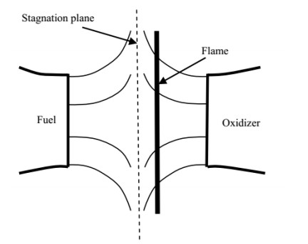
Citation: Patrick Wanjiru, Nancy Karuri, Paul Wanyeki, Paul Kioni, Josephat Tanui. Numerical simulation of the effect of diluents on NOx formation in methane and methyl formate fuels in counter flow diffusion flame[J]. AIMS Environmental Science, 2020, 7(2): 140-152. doi: 10.3934/environsci.2020008
[1] | Chun He, James C.L. Chow . Gold nanoparticle DNA damage in radiotherapy: A Monte Carlo study. AIMS Bioengineering, 2016, 3(3): 352-361. doi: 10.3934/bioeng.2016.3.352 |
[2] | Dewmini Mututantri-Bastiyange, James C. L. Chow . Imaging dose of cone-beam computed tomography in nanoparticle-enhanced image-guided radiotherapy: A Monte Carlo phantom study. AIMS Bioengineering, 2020, 7(1): 1-11. doi: 10.3934/bioeng.2020001 |
[3] | Megha Sharma, James C. L. Chow . Skin dose enhancement from the application of skin-care creams using FF and FFF photon beams in radiotherapy: A Monte Carlo phantom evaluation. AIMS Bioengineering, 2020, 7(2): 82-90. doi: 10.3934/bioeng.2020008 |
[4] | Abdulmajeed Alsufyani . Performance comparison of deep learning models for MRI-based brain tumor detection. AIMS Bioengineering, 2025, 12(1): 1-21. doi: 10.3934/bioeng.2025001 |
[5] | José Luis Calvo-Guirado, Marta Belén Cabo-Pastor, Félix de Carlos-Villafranca, Nuria García-Carrillo, Manuel Fernández-Domínguez, Francisco Martínez Martínez . Micro-CT evaluation of bone grow concept of an implant with microstructured backtaper crestally and sub-crestally placed. Preliminary study in New Zealand rabbits tibia at one month. AIMS Bioengineering, 2023, 10(4): 406-420. doi: 10.3934/bioeng.2023024 |
[6] | N. Supraja, T.N.V.K.V. Prasad, M. Soundariya, R. Babujanarthanam . Synthesis, characterization and dose dependent antimicrobial and anti-cancerous activity of phycogenic silver nanoparticles against human hepatic carcinoma (HepG2) cell line. AIMS Bioengineering, 2016, 3(4): 425-440. doi: 10.3934/bioeng.2016.4.425 |
[7] | Sarbaz H. A. Khoshnaw, Azhi Sabir Mohammed . Computational simulations of the effects of social distancing interventions on the COVID-19 pandemic. AIMS Bioengineering, 2022, 9(3): 239-251. doi: 10.3934/bioeng.2022016 |
[8] | Kristen K. Comfort . The rise of nanotoxicology: A successful collaboration between engineering and biology. AIMS Bioengineering, 2016, 3(3): 230-244. doi: 10.3934/bioeng.2016.3.230 |
[9] | Xiang-Xiang Guan, Xiao-Juan Zhu, Zhao-Hui Deng, Yu-Rong Zeng, Jie-Ru Liu, Jiang-Hua Li . The association between nicotinamide N-methyltransferase gene polymorphisms and primary hypertension in Chinese Han Population. AIMS Bioengineering, 2021, 8(2): 130-139. doi: 10.3934/bioeng.2021012 |
[10] | Jose Luis Calvo-Guirado, Nuria García Carrillo, Félix de Carlos-Villafranca, Miguel Angel Garces-Villala, Lanka Mahesh, Juan Carlos Ibanez, Francisco Martinez-Martinez . A micro-CT evaluation of bone density around two different types of surfaces on one-piece fixo implants with early loading-an experimental study in dogs at 3 months. AIMS Bioengineering, 2022, 9(4): 383-399. doi: 10.3934/bioeng.2022028 |
We consider a singular no-sign obstacle problem of the type
{div(xa1∇u)=xa1f(x)χ{u≠0}in B+1,u=0on B1∩{x1=0}, | (1.1) |
where a>1, χD is the characteristic function of D, B1⊂Rn is the unit ball and B+1=B1∩{x1>0}. The equation is considered in the weak form,
∫B+1xa1∇u∇φdx=∫B+1xa1f(x)φχ{u≠0}dx, |
for all φ∈W1,20(B+1). This problem, when the non-negativity assumption u≥0 is imposed, is already studied in [9]. The above no-sign problem, as a general semilinear PDE with non-monotone r.h.s., introduces certain difficulties and to some extent some challenges. To explain this we shall give a very short review of the existing results and methods for similar type of problems (see also the book [6] and Caffarelli's review of the classical obstacle problem [2]). The general methodology of approaching such problems lies in using the so-called ACF-monotonicity formula (see [8]) or alternatively using John Andersson's dichotomy (see [1] or [3]). Although there are still some chances that both these methods will work for our problem above, we shall introduce a third method here which relies on a softer version of a monotonicity formula (which has a wider applicability) in combination with some elaborated analysis. We refer to this as a Weiss-type monotonicity formula, see (2.1) below.
For clarity of exposition we shall introduce some notations and definitions here that are used frequently in the paper. Throughout this paper, Rn will be equipped with the Euclidean inner product x⋅y and the induced norm |x|, Br(x0) will denote the open n-dimensional ball of center x0, radius r with the boundary ∂Br(x0). In addition, Br=Br(0) and ∂Br=∂Br(0). Rn+ stands for half space {x∈Rn:x1>0} as well as B+r=Br∩Rn+. Moreover, in the text we use the n-dimensional Hausdorff measure Hn. For a multi-index μ=(μ1,⋯,μn)∈Zn+, we denote the partial derivative with ∂μu=∂μ1x1⋯∂μnxnu and |μ|1=μ1+⋯+μn.
For a domain Ω⊂Rn+ and 1≤p<∞, we use the notation Lp(Ω) and Wm,p(Ω) as the standard spaces. However, we need some new notation for the weighted spaces
Lp(Ω;xθ1):={u:∫Ωxθ1|u(x)|pdx<∞}, |
where θ∈R. For m∈N, we define the weighted Sobolev space Wm,p(Ω;xθ1) as the closure of C∞(¯Ω) with the following norm,
‖u‖Wm,p(Ω;xθ1):=‖u‖Lp(Ω;xθ1)+‖x1Du‖Lp(Ω;xθ1)+⋯+‖xm1Dmu‖Lp(Ω;xθ1). |
It is noteworthy that for θ=0, we have Lp(Ω;1)=Lp(Ω) but Wm,p(Ω;1)⊋Wm,p(Ω). Generally, the trace operator has no sense for θ>−1, while functions in W1,p(Ω;xθ1) have zero traces on {x1=0} for θ≤−1. (Theorem 6 in [7]).
We consider u∈W1,p(B+1,xθ1) for some θ<−n and n<p to be a weak solution of (1.1). This condition provides the continuity of x(θ+n)/p1u up to the boundary according to Sobolev embedding Theorem 3.1 in [5]. First, we prove the following a priori regularity result.
Proposition 1.1. (Appendix A) Let u∈W1,p(B+1,xθ1) be a solution of (1.1) for some θ<−n, n<p and f∈L∞(B+1). Then for each max{0,1+θ+np}<β<1 there exists C=C(β,n,a) such that for r≤1/2,
supB+r(x0)|xβ−11u|≤Cr2β, |
for all x0∈{x1=0}.
In Appendix A we will prove this proposition. Our main result in this paper concerns the optimal growth rate of solution u of (1.1) at touching free boundary points, which is stated in the following theorem.
Theorem 1.2. Suppose u∈W1,p(B+1,xθ1) is a solution of (1.1) for some θ<−n, n<p and x0∈∂{u=0}∩{x1=0}∩B+1/4. Moreover, if f∈Cα(¯B+1) for some α∈(0,1), then
|u(x)|≤Cx21((|x−x0|+x1x1)(n+a+4)/2+1), |
for a universal constant C=C(a,n,[f]0,α).
Our main tool in proving optimal decay for solutions from the free boundary points is Weiss-monotonicity formula, combined with some elaborated techniques. We define the balanced energy functional
Φx0(r,u)=r−n−2−a∫B+r(x0)(xa1|∇u|2+2xa1f(x0)u)dx−2r−n−3−a∫∂Br(x0)∩Rn+xa1u2dHn−1. | (2.1) |
Considering the scaling ur,x0=ur(x)=u(rx+x0)r2, Φx0(r,u)=Φ0(1,ur). In what follows we prove almost-monotonicity of the energy.
Lemma 2.1 (Almost-Monotonicity Formula). Let u solve (1.1) and be as in Proposition 1.1 and assume that ∇u(x0)=0 for some x0∈{x1=0} and f∈Cα(¯B+1) for some α∈(0,1). Then u satisfies, for r≤r0 such that B+r0(x0)⊆B+1,
ddrΦx0(r,u)≥2r∫∂B1∩Rn+xa1(∂rur)2dHn−1−Crα+β−2, |
where C depends only on ‖f‖Cα(¯B+1) and the constant C(β,n,a) in Proposition 1.1.
Proof. Let ur(x):=u(rx+x0)r2, then
=12ddrΦx0(r,u)=12ddr[∫B+1(xa1|∇ur|2+2xa1f(x0)ur)dx−2∫∂B1∩Rn+xa1u2rdHn−1]=12[∫B+1(2xa1∇ur⋅∇∂rur+2xa1f(x0)∂rur)dx−4∫∂B1∩Rn+xa1ur∂rurdHn−1]=∫B+1div(xa1∂rur∇ur)−∂rurdiv(xa1∇ur)+xa1f(x0)∂rurdx−2∫∂B1∩Rn+xa1ur∂rurdHn−1=∫B+1(f(x0)−f(rx+x0)χ{ur≠0})xa1∂rurdx+∫∂B+1xa1∂rur∇ur⋅νdHn−1−2∫∂B1∩Rn+xa1ur∂rurdHn−1=∫B+1(f(x0)−f(rx+x0)χ{ur≠0})xa1∂rurdx+r∫∂B1∩Rn+xa1(∂rur)2dHn−1=∫B+1(f(x0)−f(rx+x0))χ{ur≠0}xa1∂rurdx+f(x0)∫B+1∩{ur=0}xa1∂rurdx+r∫∂B1∩Rn+xa1(∂rur)2dHn−1. |
Note that the second integral
∫B+1∩{ur=0}xa1∂rurdx=0 |
as |{ur=0∧∇ur≠0}|=0 and ∂rur=0 on {ur=0∧∇ur=0}. Since |∂rur|≤Crβ−2 we infer that
∫B+1(f(x0)−f(rx+x0))χ{ur≠0}xa1∂rurdx≥−Crα+β−2 |
and conclude that
12ddrΦx0(r,u)≥r∫∂B1∩Rn+xa1(∂rur)2dHn−1−Crα+β−2. |
Definition 2.2. Let HP2 stand for the class of all two-homogeneous functions P∈W1,2(B+1;xa−21) satisfying div(xa1∇P)=0 in Rn+ with boundary condition P=0 on x1=0. We also define the operator Π(v,r,x0) to be the projection of vr,x0 onto HP2 with respect to the inner product
⟨vw⟩=∫∂B1∩n+xa1vwdHn−1. |
We will use the following extension of [10,Lemma 4.1].
Lemma 2.3. Assume that div(xa1∇w)=0 in B+1 with boundary condition w=0 on x1=0, and w(0)=|∇w(0)|=0. Then
∫B+1xa1|∇w|2dx−2∫∂B1∩Rn+xa1w2dHn−1≥0, |
and equality implies that w∈HP2, i.e., it is homogeneous of degree two.
Proof. We define an extension of the Almgren frequency,
r↦N(w,r):=r∫B+rxa1|∇w|2dx∫∂B+rxa1w2dHn−1, |
12N′(w,r)N(w,r)=∫∂B+rxa1(∂νw)2dHn−1∫∂B+rxa1w∂νwdHn−1−∫∂B+rxa1w∂νwdHn−1∫∂B+rxa1w2dHn−1≥0. |
Moreover, if N(w,r)=κ for ρ<r<σ, it implies that w is homogeneous of degree κ in Bσ∖Bρ.
Now supposing towards a contradiction that N(w,s)<2 for some s∈(0,1], and defining wr(x):=w(rx)‖w(rx)‖L2(∂B+1,xb1), we infer from N(w,s)<2 that ∇wr is bounded in L2(B+1;xa1) and so ∇wrm⇀∇w0 weakly in L2(B+1;xa1) and wrm→w0 strongly in L2(∂B+1;xa1) as a sequence rm→0. Consequently, w0 satisfies div(xa1∇w0)=0 in B+1, w0(0)=|∇w0(0)|=0 and w0=0 on x1=0 as well as ‖w0‖L2(∂B+1;xa1)=1. Furthermore, for all r∈(0,1) we have
N(w0,r)=limrm→0N(wrm,r)=limrm→0N(w,rrm)=N(w,0+), |
and so w0 must be a homogeneous function of degree κ:=N(w,0+)<2. Note that for every multi-index μ∈{0}×Zn−1+, the higher order partial derivative ζ=∂μw0 satisfies the equation div(xa1∇ζ)=0 in Rn+. From the integrability and homogeneity we infer that ∂μw0≡0 for κ−|μ|1<−n2, otherwise
∫B+1|∂μw0|2dx=(∫10r2(κ−|μ|1)+n−1dr)∫∂B1∩Rn+|∂μw0|2dHn−1 |
can not be bounded. Thus x′↦w0(x1,x′) is a polynomial, and we can write w0(x1,x′)=xκ1p(x′x1). Consider the multi-index μ such that |μ|1=degp, so ∂μw0=xκ−|μ|11∂μp is a solution of div(xa1∇ζ)=0 in Rn+. Therefore, ∂μw0∈W1,2(B+1;xθ1) for −1<θ according to Proposition A.1, which implies that 2(κ−|μ|1)+θ>−1. So, degp<κ+θ+12.
Substituting w0(x)=xκ−11(αx1+ℓ⋅x′) for κ>1 in the equation and comparing with w0(0)=|∇w0(0)|=0 we arrive at the only nonzero possible case being κ+a=2, which contradicts a>1. The case κ<1 leads to degp=0 and w0(x)=αxκ1, which implies κ+a=1 and a contradiction to a>1.
Proposition 3.1. Let f∈Cα(¯B+1) and u be solution of (1.1) satisfying the condition in Proposition 1.1. Then the function
r↦r−n−3−a∫∂B+r(x0)xa1u2(x)dHn−1 |
is bounded on (0,1/8), uniformly in x0∈∂{u=0}∩{x1=0}∩B1/8.
Proof. Let us divide the proof into steps.
Step 1 We claim that there exists a constant C1<∞ such that for all x0∈∂{u=0}∩{x1=0}∩B1/8 and r≤1/8,
f(x0)∫B+1xa1ux0,r(x)dx≥−C1, |
where ux0,r:=u(rx+x0)r2. To prove this we observe that w:=ux0,r satisfies
div(xa1∇w)=xa1fr(x):=xa1f(x0+rx)χ{ux0,r≠0},in B+1. |
Moreover, for ϕ(ρ):=ρ−n−a+1∫∂B+ρxa1w(x)dHn−1 we have
ϕ′(ρ)=∫∂B+1xa1∇w(ρx)⋅xdHn−1=ρ−n−a+1∫B+ρdiv(xa1∇w(x))dx=ρ−n−a+1∫B+ρxa1fr(x)dx. |
If f(x0)≥18α[f]0,α then fr≥0 for r≤1/8. Therefore ϕ is increasing and ϕ(ρ)≥ϕ(0)=0 (recall that w(0)=0). Similarly, if f(x0)≤−18α[f]0,α, we obtain that ϕ(ρ)≤0. Therefore the claim is true for C1=0 in these cases.
In the case |f(x0)|≤18α[f]0,α, then |fr(x)|≤28α[f]0,α and then
|ϕ′(ρ)|≤21−3α[f]0,αρ−n−a+1∫B+ρxa1dx≤21−3α[f]0,αρ. |
So, |ϕ(ρ)|≤2−3α[f]0,αρ2 and
|f(x0)∫B+1xa1ux0,r(x)dx|=|f(x0)∫10ρn+a−1ϕ(ρ)dρ|≤2−6α[f]20,αn+a+2=:C1. |
Step 2 We claim that there exists a constant C2<∞ such that
distL2(∂B1∩Rn+;xa1)(ux0,r,HP2)≤C2, |
for every x0∈∂{u=0}∩{x1=0}∩B1/8, r≤1/8. Suppose towards a contradiction that this is not true, then there exists a sequence um, xm→ˉx and rm→0 such that
Mm=‖umxm,rm−Π(um,rm,xm)‖L2(∂B1∩Rn+;xa1)→∞,m→∞. |
Let um:=umxm,rm and pm=Π(um,rm,xm) and wm=um−pmMm. Then, since um(0)=|∇um(0)|=0 and by the monotonicity formula and the result of previous step, we find that
∫B+1xa1|∇wm|2dx−2∫∂B+1xa1w2mdHn−1=1M2m[Φxm(rm)−2∫B+1f(xm)xa1umdx]+1M2m∫∂B+1xa1(pm∇pm⋅ν−2um∇pm⋅ν−2p2m+4umpm)dHn−1≤1M2m(Φxm(rm)+2C1)≤1M2m(Φxm(12)+2C1)→0,m→∞. | (3.1) |
Passing to a subsequence such that ∇wm⇀∇w in L2(B+1;xa1) as m→∞, the compact embedding on the boundary implies that ‖w‖L2(∂B1∩Rn+;xa1)=1, and
∫B+1xa1|∇w|2dx≤2∫∂B1xa1w2dHn−1 | (3.2) |
and that
∫∂B1wpdHn−1=0,∀p∈HP2. | (3.3) |
Since div(xa1∇wm)=x1Mmf(xm+r⋅)χ{um≠0}, it follows that div(xa1∇w)=0 in B+1. Moreover, we obtain from Lp-theory that wm→w in C1,αloc(B+1) for each α∈(0,1) as m→∞. Consequently w(0)=|∇w(0)|=0. Thus we can apply Lemma 2.3 and obtain from (3.2) that w is homogeneous of degree 2, contradicting (3.3) and ‖w‖L2(∂B1)=1. This proves the claim.
Step 3 We will show that there exists constant C2 such that for all x0∈∂{u=0}∩{x1=0} satisfying
lim infr→0+|B+r(x0)∩{u=0}||B+r|=0, | (3.4) |
we have
Φx0(0+)−∫B+1xa1f(x0)ux0,rdx≥−C2rα|f(x0)|. |
In order to see this, we can observe that
∫B+1xa1f(x0)ux0,r(x)dx=f(x0)∫10∫10∂s[∫∂B+ρ(sx1)aux0,r(sx)dHn−1(x)]dsdρ=f(x0)∫10ρ∫10∫∂B+ρ(sx1)a∇ux0,r(sx)⋅νdHn−1dsdρ=f(x0)∫10ρ∫10s∫B+ρdiv((sx1)a∇ux0,r(sx))dxdsdρ=f(x0)∫10ρ∫10s∫B+ρ(sx1)af(rsx)χΩx0,r(sx)dxdsdρ=f(x0)2∫10ρ1+a+n∫10s1+a∫B+1xa1dxdsdρ+f(x0)∫10ρ1+a+n∫10s1+a∫B+1xa1(f(rsρx)−f(x0))dxdsdρ≤f(x0)2(n+a+2)(a+2)∫B+1xb1dx+C2rα|f(x0)|. |
Now by condition (3.4), consider a sequence rm→0 such that |B+rm(x0)∩{v=0}||B+rm|→0 and assume that ∇(ux0,rm−px0,rm)⇀∇w in L2(B+1;xa1) as m→∞. Observe now div(xa1w)=f(x0) in B+1 and by similar calculation as above we will have
∫B+1xa1f(x0)wdx=f(x0)2(n+a+2)(a+2)∫B+1xa1dx. |
On the other hand,
Φx0(0+)=limm→∞Φx0(rm)≥∫B+1(xa1|∇w|2+2f(x0)xa1w)dx−2∫∂B+1xa1w2dHn−1=∫B+1(−wdiv(xa1∇w)+2f(x0)xa1w)dx=∫B+1xa1f(x0)wdx=f(x0)2(n+a+2)(a+2)∫B+1xa1dx. |
Step 4 In this step, we prove the proposition for the points satisfying condition (3.4). For these points, we have
12∂r[∫∂B+1xa1u2x0,rdHn−1]=∫∂B+1xa1ux0,r∂rux0,rdHn−1=1r∫∂B+1xa1ux0,r(∇ux0,r⋅x−2ux0,r)dHn−1=1r∫B+1(xa1|∇ux0,r|2+ux0,rdiv(xa1∇ux0,r))dx−2r∫∂B+1xa1u2x0,rdHn−1=1r(Φx0(r)−2∫B+1f(x0)xa1ux0,r(x)dx+∫B+1xa1f(rx)ux0,r(x)dx)=1r(Φx0(r)−∫B+1f(x0)xa1ux0,rdx)+1r(∫B+1(f(rx)−f(x0))xa1ux0,r(x)dx)≥1r(Φx0(0+)−∫B+1f(x0)xa1ux0,rdx)−Crα+β−2−C3rα+β−2≥−C2rα−1−Crα+β−2−C3rα+β−2 |
Thus r↦∂r[∫∂B+1xa1u2x0,rdHn−1] is integrable and we obtain uniform boundedness of ∫∂B+1xa1u2x0,rdHn−1=r−n−3−b∫∂Br(x0)+xa1u2dHn−1 for all points with property (3.4). It follows that the boundedness holds uniformly on the closure of those points x0.
Step 5 We now consider the case
\liminf\limits_{r\to0^{+}}\frac{|B_r^+(x^0)\cap\{u = 0\}| }{|B_r^+|} \gt 0. |
Let us assume towards a contradiction that there are sequences u^m , r_{m} and x^m such that and M_{m} = \|{u_{x^m, r_m}}\|_{ {\mathcal L}^{2}(\partial B_{1}^+)}\to+\infty as m\to\infty . Setting w_{m} = \frac{u^m_{x^m, r_{m}}}{M_{m}} we obtain, as in Step 2, that a subsequence of w_{m} converges weakly in W^{1, 2}(B_{1}^+; x_1^{a-2}) to a function w , with \|w_\|{ {\mathcal L}^{2}(\partial B_{1}^+; x_1^a)} = 1 , w(0) = \lvert\nabla w(0)\rvert = 0 , \operatorname{div}(x_1^a\nabla w) = 0 and
\int_{B_{1}^+}x_1^a\lvert\nabla w|^{2}dx\le2\int_{\partial B_{1}^+}x_1^aw^{2}{\mathop{}\!d} {\mathcal H}^{n-1}. |
According to Lemma 2.3, w\in\mathbb{HP}_2 . In addition we now know that
\int_{B_{1}^+}\chi_{\{w = 0\}}\ge\limsup\limits_{r_{m}\to0^{+}}\int_{B_{1}^+}\chi_{\{u_{x^0,r_{m}} = 0\}} \gt 0. |
This however contradicts the analyticity of w inside B_1^+ , knowing that \|w_\|{ {\mathcal L}^{2}(\partial B_{1};x_1^a)} = 1 .
Now we are ready to prove the main result of the article.
Proof of Theorem 1.2. From Theorem 8.17 in [4], we know that if \operatorname{div}(b(x)\nabla w) = g such that 1\leq b(x)\leq 5^a , then there exists a universal constant C = C(a, n) such that
\|w\|_{ {\mathcal L}^\infty(B_{R/2})}\leq C(a,n)\left(R^{-n/2}\|w\|_{ {\mathcal L}^2(B_R)}+R^{2}\|g\|_{ {\mathcal L}^\infty(B_R)}\right). |
Now for x^0 \in \partial\{u = 0\}\cap\{x_1 = 0\}\cap B_{1/8}^+ and an arbitrary point y\in \partial B_r^+(x^0) , we apply the above estimate for R = 2\delta/3 , w = (\delta/3)^au and equation \operatorname{div}\left(b(x)\nabla w\right) = x_1^af\chi_{\{u\neq0\}} , where \delta = y_1 and b(x) = \frac{x_1^a}{(\delta/3)^a} . Note that 1\leq b(x)\leq 5^a in B_{2\delta/3}(y) and
|u(y)|\leq C(a,n)\left((2\delta/3)^{-n/2}\|u\|_{ {\mathcal L}^2(B_{2\delta/3}(y))}+(2\delta/3)^{2}5^a\|f\|_{ {\mathcal L}^\infty(B_{2\delta/3}(y))}\right). |
According to Proposition 3.1,
\begin{align*} \|u\|^2_{ {\mathcal L}^2(B_{2\delta/3}(y))}\leq & \Big(\frac3\delta\Big)^a\int_{B_{2\delta/3}(y)}x_1^a|u|^2\,dx\\ \leq & \Big(\frac3\delta\Big)^a\int_{B_{r+2\delta/3}(x^0)}x_1^a|u|^2\,dx \\ \leq &C\Big(\frac3\delta\Big)^a(r+2\delta/3)^{n+a+4}. \end{align*} |
Hence,
\begin{equation*} |u(y)|\leq C\left(\delta^{-(n+a)/2}(r+\delta)^{(n+a+4)/2}+\delta^{2}\right)\leq Cy_1^2\left(\Big(\frac{r+y_1}{y_1}\Big)^{(n+a+4)/2}+1\right). \end{equation*} |
From this theorem it follows that solutions have quadratic growth inside cones.
Corollary 3.2. Suppose u is a solution of (1.1) satisfying the condition in Proposition 1.1 and x^0\in \partial\{u = 0\}\cap\{x_1 = 0\}\cap B_{1/8}^+ . Then, for every constant \tau > 0 ,
\sup\limits_{B_r(x^0)\cap {\mathcal C}}|u|\leq C\left(\left(\frac{1}{\tau}+ 1\right)^{\frac{n+a+4}{2}}+1\right) r^2, |
where {\mathcal C} : = \{x: x_1\geq \tau |x-x^0|\} .
This paper was prepared while M. Fotouhi was visiting KTH Royal Institute of Technology. A. Minne was supported by the Knut and Alice Wallenberg Foundation. H. Shahgholian was supported by Swedish Research Council.
The authors declare no conflict of interest.
Let u be a solution of (1.1) for f\in {\mathcal L}^\infty(B_1^+) . We are going to show a priori regularity for solutions to (1.1). Consider the operator {\mathcal L}_{a, c}u: = x_1^2\Delta u+ax_1\partial_1u-cu . The following proposition is the regularity result related to this operator which has been proven by Krylov [5,Theorem 2.7,Theorem 2.8].
Proposition A.1. i) For any a\in {\mathbb R}, p > 1 and \theta\in {\mathbb R} there exists a constant c_0 > 0 such that for any c\geq c_0 the operator {\mathcal L}_{a, c} is a bounded one-to-one operator from W^{2, p}({\mathbb R}^n_+; x_1^\theta) onto {\mathcal L}^p({\mathbb R}^n_+; x_1^\theta) and its inverse is also bounded, in particular for any u\in W^{2, p}({\mathbb R}^n_+; x_1^\theta)
\|u\|_{W^{2,p}( {\mathbb R}^n_+;x_1^\theta)}\leq C\| {\mathcal L}_{a,c}u\|_{ {\mathcal L}^p( {\mathbb R}^n_+;x_1^\theta)}, |
where C is independent of u and c .
ii) The statement in i) is valid for the operator {\mathcal L}_{a, 0} when -1 < \theta < a-2 and a > 1 or either a-2 < \theta < -1 and a < 1 .
Now we can deduce a priori regularity result for u as follows.
Proof of Proposition 1.1. Notice that x_1^{\beta-1}u\in C(\overline{B_1^+}) due to Sobolev embedding Theorem 3.1 in [5]. Then if the statement of proposition fails, there exists a sequence u_j of solutions (1.1), x^j\in \{x_1 = 0\} and r_j\rightarrow0 such that
\sup\limits_{B_r^+(x^j)}|x_1^{\beta-1}u_j|\leq jr^{1+\beta/2},\quad \forall r\geq r_j, \qquad \sup\limits_{B_{r_j}^+(x^j)}|x_1^{\beta-1}u_j| = jr_j^{1+\beta/2}. |
In particular, the function \tilde u_j(x) = \frac{u_j(x^j+r_jx)}{jr_j^{1+\beta/2}} , satisfies
\begin{equation} \sup\limits_{B_R^+}|x_1^{\beta-1}\tilde u_j|\leq R^{1+\beta/2}, \qquad\text{for }1\leq R\leq\frac1{r_j}, \end{equation} | (A.1) |
and with equality for R = 1 , along with
\begin{equation} {\mathcal L}_{a,c_0}\tilde u_j = \frac{r_j^{1-\beta/2}}{j}f(x^j+r_jx)-c_0\tilde u_j, \end{equation} | (A.2) |
where c_0 is defined in Proposition A.1. According to (A.1), the right hand side of (A.2) is uniformly bounded in {\mathcal L}^p(B_R^+; x_1^\theta) for p(\beta-1)-1 < \theta\leq-1 . From here and Proposition A.1 we conclude that \{\tilde u_j\} is bounded in W^{2, p}(B_{R}^+; x_1^\theta) for some \theta\leq-1 and there is a convergent subsequence, tending to a function u_0 with properties
\begin{equation} \sup\limits_{B_R^+}|x_1^{\beta-1} u_0|\leq R^{1+\beta/2},\quad\forall R\geq1,\quad\sup\limits_{B_1^+}|x_1^{\beta-1} u_0| = 1,\quad \operatorname{div}(x_1^a \nabla u_0) = 0, \end{equation} | (A.3) |
as well as the condition \theta\leq-1 insures that the trace operator is well defined and u_0 is zero on \{x_1 = 0\} . The Liouville type theorem in [9,Lemma 20]) implies that
|D^2u_0(x^0)|\leq \frac C{R^2}\sup\limits_{B_R^+(x^0)}|u_0|\leq \frac{C(R+|x_0|)^{2-\beta/2}}{R^2}\rightarrow0. |
Therefore, u_0 is a linear function, which contradicts (A.3).
[1] |
Basha SA, KR Gopal, S Jebaraj (2009) A review on biodiesel production, combustion, emissions and performance. Renew Sus energ Rev 13: 1628-1634. doi: 10.1016/j.rser.2008.09.031
![]() |
[2] | Abed K, M Gad, A El Morsi, et al. (2019) Effect of biodiesel fuels on diesel engine emissions. Egypt J Petrol 34:198-223. |
[3] | Liu HP, S Strank, M Werst, et al. (2010) Combustion emissions modeling and testing of neat biodiesel fuels. in ASME 2010 4th International Conference on Energy Sustainability. ASME Digit Collect 2010: 131-140. |
[4] | Ekarong S (2013) Synergistic effects of alcohol-based renewable fuels: fuel properties and emissions. Ph. D. thesis, University of Birmingham. |
[5] | Graboski MS, RL McCormick, TL Alleman, et al. (1999) Effect of biodiesel composition on NOx and PM emissions from a DDC Series 60 engine. Report for National Renewable Energy Laboratory. |
[6] | Dooley S, Chaos M, Burke MP, et al. (2009) An experimental and kinetic modeling study of methyl formate oxidation. Proceedings of the European Combustion Meeting. |
[7] |
Dooley S, Dryer FL, Yang B, et al. (2011) An experimental and kinetic modeling study of methyl formate low-pressure flames. Combust Flame 158: 732-741. doi: 10.1016/j.combustflame.2010.11.003
![]() |
[8] | Kioni PN, Tanui JK, Gitahi A (2013) Numerical simulations of nitric oxide (NO) formation in methane, methanol and methyl formate in different flow configurations. J Clean Energ Tech 1. |
[9] | Tanui J, PN Kioni, A Gitahi (2014) Numerical Simulation of Nitric Oxide (NO) Formation in Methane, Methanol and Methyl Formate in a Homogeneous System. J Sust Res Engin 1. |
[10] | Ngugi JM, Kioni PN, Tanui JK (2018) Numerical Study of Nitrogen Oxides (NOx) Formation in Homogenous System of Methane, Methanol and Methyl Formate at High Pressures. J Clean Energ Tech 6. |
[11] |
Saleh H (2009) Effect of exhaust gas recirculation on diesel engine nitrogen oxide reduction operating with jojoba methyl ester. Renew Energ 34: 2178-2186. doi: 10.1016/j.renene.2009.03.024
![]() |
[12] |
Kumar BR, S Saravanan, D Rana, et al. (2016) Effect of a sustainable biofuel-n-octanol-on the combustion, performance and emissions of a DI diesel engine under naturally aspirated and exhaust gas recirculation (EGR) modes. Energ Convers Manage 118: 275-286. doi: 10.1016/j.enconman.2016.04.001
![]() |
[13] |
Pedrozo VB, I May, H Zhao (2017) Exploring the mid-load potential of ethanol-diesel dual-fuel combustion with and without EGR. Appl Energ 193: 263-275. doi: 10.1016/j.apenergy.2017.02.043
![]() |
[14] |
Shi X, B Liu, C Zhang, et al. (2017) A study on combined effect of high EGR rate and biodiesel on combustion and emission performance of a diesel engine. Appl Therm Eng 125: 1272-1279. doi: 10.1016/j.applthermaleng.2017.07.083
![]() |
[15] |
Drake MC, RJ Blint (1991) Calculations of NOx formation pathways in propagating laminar, high pressure premixed CH4/air flames. Combust Sci Tech 75: 261-285. doi: 10.1080/00102209108924092
![]() |
[16] | Pillier L, P Desgroux, B Lefort, et al. (2006) NO prediction in natural gas flames using GDF-Kin® 3.0 mechanism NCN and HCN contribution to prompt-NO formation. Fuel 85: 896-909. |
[17] |
Tsuji H (1982) Counterflow diffusion flames. Prog Energ Combust Sci 8: 93-119. doi: 10.1016/0360-1285(82)90015-6
![]() |
[18] |
Barlow R, A Karpetis, J Frank, et al. (2001) Scalar profiles and NO formation in laminar opposed-flow partially premixed methane/air flames. Combust Flame 127: 2102-2118. doi: 10.1016/S0010-2180(01)00313-3
![]() |
[19] | Goos E, A Burcat, B Ruscic (2012) Extended third millennium thermodynamic database for combustion and air-pollution use with updates from active thermochemical tables. Burcat und B. Ruscic, Third Millennium Ideal Gas Condensed Phase Thermochemical Database for Combustion with Updates from Active Thermochemical Tables, Joint Report: ANL-05/20, Argonne National Laboratory, Argonne, IL, USA, TAE. 960. |
[20] |
Li W, Z Liu, Z Wang, et al. (2014) Experimental investigation of the thermal and diluent effects of EGR components on combustion and NOx emissions of a turbocharged natural gas SI engine. Energ Conve Man 88: 1041-1050. doi: 10.1016/j.enconman.2014.09.051
![]() |
[21] | Zelenka P, H Aufinger, W Reczek, et al. (1998) Cooled EGR-a key technology for future efficient HD diesels. SAE Technical Paper. |
[22] | Version C (2009) 3, Rotexo-Cosilab GmbH & Co. KG, Bad Zwischenahn, Germany. |
[23] |
Hughes K, T Turányi, A Clague, et al. (2001) Development and testing of a comprehensive chemical mechanism for the oxidation of methane. Int J Chem Kinet 33: 513-538. doi: 10.1002/kin.1048
![]() |
[24] | Hu B, H Yong (2011) Theoretical analysis of lowest limits of NOx formation of methane-air mixtures. in Asia-Pacific Power and Energy Engineering Conference. IEEE. |
[25] | Gomaa M, A Alimin, K Kamaruddin (2011) The effect of EGR rates on NOX and smoke emissions of an IDI diesel engine fuelled with Jatropha biodiesel blends. Int J Energ Environ 2: 477-490. |
[26] |
Maiboom A, X Tauzia (2011) NOx and PM emissions reduction on an automotive HSDI Diesel engine with water-in-diesel emulsion and EGR: An experimental study. Fuel 90: 3179-3192. doi: 10.1016/j.fuel.2011.06.014
![]() |