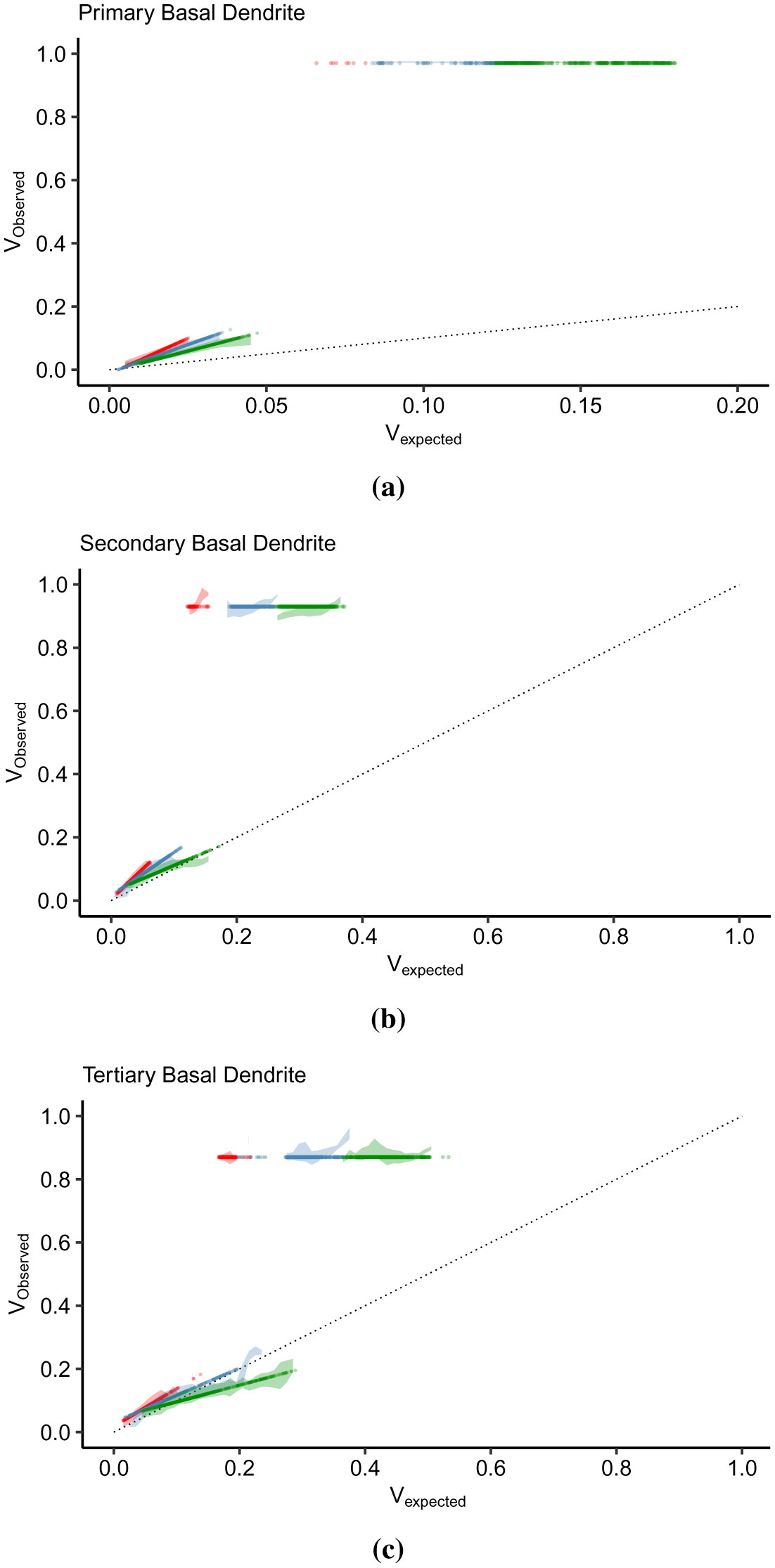
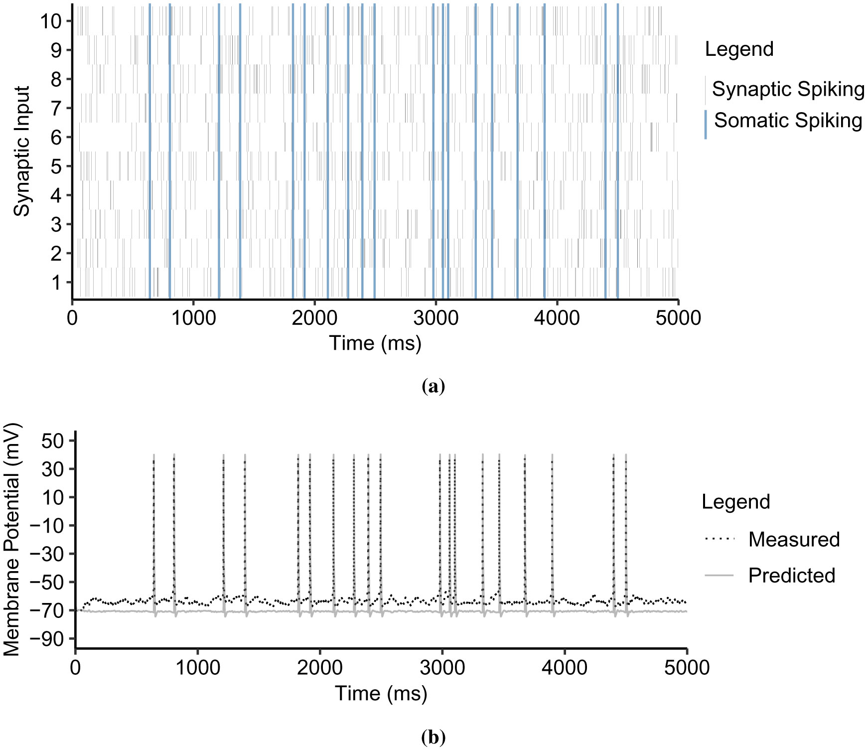
Advances in neuronal studies suggest that a single neuron can perform integration functions previously associated only with neuronal networks. Here, we proposed a dendritic abstraction employing a dynamic thresholding function that models the spatiotemporal dendritic integration process of a CA3 pyramidal neuron. First, we developed an input-output quantification process that considers the natural neuronal response and the full range of dendritic dynamics. We analyzed the IO curves and demonstrated that dendritic integration is branch-specific and dynamic rather than the commonly employed static nonlinearity. Second, we completed the integration model by creating a dendritic abstraction incorporating the spatiotemporal characteristics of the dendrites. Furthermore, we predicted the dendritic activity in each dendritic layer and the corresponding somatic firing activity by employing the dendritic abstraction in a multilayer-multiplexer information processing scheme comparable to a neuronal network. The subthreshold activity influences the suprathreshold regions via its dynamic threshold, a parameter that is dependent not only on the driving force but also on the number of activated synapses along the dendritic branch. An individual dendritic branch performs multiple integration modes by shifting from supralinear to linear then to sublinear. The abstraction includes synaptic input location-dependent voltage delay and decay, time-dependent linear summation, and dynamic thresholding function. The proposed dendritic abstraction can be used to create multilayer-multiplexer neurons that consider the spatiotemporal properties of the dendrites and with greater computational capacity than the conventional schemes.
Citation: Jhunlyn Lorenzo, Stéphane Binczak, Sabir Jacquir. A multilayer-multiplexer network processing scheme based on the dendritic integration in a single neuron[J]. AIMS Neuroscience, 2022, 9(1): 76-113. doi: 10.3934/Neuroscience.2022006
Advances in neuronal studies suggest that a single neuron can perform integration functions previously associated only with neuronal networks. Here, we proposed a dendritic abstraction employing a dynamic thresholding function that models the spatiotemporal dendritic integration process of a CA3 pyramidal neuron. First, we developed an input-output quantification process that considers the natural neuronal response and the full range of dendritic dynamics. We analyzed the IO curves and demonstrated that dendritic integration is branch-specific and dynamic rather than the commonly employed static nonlinearity. Second, we completed the integration model by creating a dendritic abstraction incorporating the spatiotemporal characteristics of the dendrites. Furthermore, we predicted the dendritic activity in each dendritic layer and the corresponding somatic firing activity by employing the dendritic abstraction in a multilayer-multiplexer information processing scheme comparable to a neuronal network. The subthreshold activity influences the suprathreshold regions via its dynamic threshold, a parameter that is dependent not only on the driving force but also on the number of activated synapses along the dendritic branch. An individual dendritic branch performs multiple integration modes by shifting from supralinear to linear then to sublinear. The abstraction includes synaptic input location-dependent voltage delay and decay, time-dependent linear summation, and dynamic thresholding function. The proposed dendritic abstraction can be used to create multilayer-multiplexer neurons that consider the spatiotemporal properties of the dendrites and with greater computational capacity than the conventional schemes.
AMPA Receptor
Action Potential
Generalized Linear Model
Input-Output
Leaky-Integrate and Fire
Linear-Nonlinear Poisson
N-methyl-D-aspartate
NMDA Receptor
Spike-timing dependent plasticity

| [1] |
Sardi S, Vardi R, Goldental A, et al. (2018) Dendritic Learning as a Paradigm Shift in Brain Learning. ACS Chem Neurosci 9: 1230-1232. https://doi.org/10.1021/acschemneuro.8b00204 
|
| [2] |
Li S, Liu N, Zhang X, et al. (2014) Bilinearity in spatiotemporal integration of synaptic inputs. PLoS Comput Biol 10: e1004014. https://doi.org/10.1371/journal.pcbi.1004014
|
| [3] |
Hao J, Wang X, Dan Y, et al. (2009) An arithmetic rule for spatial summation of excitatory and inhibitory inputs in pyramidal neurons. P Natl Acad Sci 106: 21906-21911. https://doi.org/10.1073/pnas.0912022106
|
| [4] |
Brunel N, Hakim V, Richardson M (2014) Single neuron dynamics and computation. Curr Opin Neurobiol 25: 149-155. https://doi.org/10.1016/j.conb.2014.01.005
|
| [5] |
Behabadi B, Polsky A, Jadi M, et al. (2012) Location-dependent excitatory synaptic interactions in pyramidal neuron dendrites. PLoS Comput Biol 8: e1002599. https://doi.org/10.1371/journal.pcbi.1002599
|
| [6] |
Li S, Liu N, Zhang X, et al. (2019) Dendritic computations captured by an effective point neuron model. P Natl Acad Sci 116: 15244-15252. https://doi.org/10.1073/pnas.1904463116
|
| [7] |
Payeur A, Béque J-C, Naud R (2019) Classes of dendritic information processing. Curr Opin Neurobiol 58: 78-85. https://doi.org/10.1016/j.conb.2019.07.006
|
| [8] |
Rall W (1962) Theory of physiological properties of dendrites. Ann NY Acad Sci 96: 1071-1092. https://doi.org/10.1111/j.1749-6632.1962.tb54120.x
|
| [9] | Rall W, Reiss R (1964) Neural theory and modeling. Stanford: Stanford Univ. Press p. 78. |
| [10] |
Stuart G, Spruston N (2015) Dendritic integration: 60 years of progress. Nat Neurosci 18: 1713-1721. https://doi.org/10.1038/nn.4157
|
| [11] | Poirazi P, Papoutsi A (2020) Illuminating dendritic function with computational models. Nat Rev Neurosci 1–19. https://doi.org/10.1038/s41583-020-0301-7 |
| [12] |
Gleeson P, Cantarelli M, Marin B, et al. (2019) Open source brain: a collaborative resource for visualizing, analyzing, simulating, and developing standardized models of neurons and circuits. Neuron 103: 395-411. https://doi.org/10.1016/j.neuron.2019.05.019
|
| [13] |
McCulloch W, Pitts W (1943) A logical calculus of the ideas immanent in nervous activity. B Math Biophy 5: 115-133. https://doi.org/10.1007/BF02478259
|
| [14] |
Weber A, Pillow J (2017) Capturing the dynamical repertoire of single neurons with generalized linear models. Neural Comput 29: 3260-3289.
|
| [15] |
Wang Y, Liu S-C (2010) Multilayer processing of spatiotemporal spike patterns in a neuron with active dendrites. Neural Comput 22: 2086-2112. https://doi.org/10.1162/neco.2010.06-09-1030
|
| [16] |
Ujfalussy B, Makara J, Lengyel M, et al. (2018) Global and multiplexed dendritic computations under in vivo-like conditions. Neuron 100: 579-592. https://doi.org/10.1016/j.neuron.2018.08.032
|
| [17] |
Poirazi P, Brannon T, Mel B (2003) Pyramidal neuron as two-layer neural network. Neuron 37: 989-999. https://doi.org/10.1016/S0896-6273(03)00149-1
|
| [18] | Zhang D, Li Y, Rasch M, et al. (2013) Nonlinear multiplicative dendritic integration in neuron and network models. Front Comput Neurosc 7: 56. https://doi.org/10.3389/fncom.2013.00056 |
| [19] |
Jadi M, Behabadi B, Poleg-Polsky A, et al. (2014) An augmented two-layer model captures nonlinear analog spatial integration effects in pyramidal neuron dendrites. P IEEE 102: 782-798. https://doi.org/10.1109/JPROC.2014.2312671
|
| [20] |
Polsky A (2004) Computational subunits in thin dendrites of pyramidal cells. Nat Neurosci 7: 621-627. https://doi.org/10.1038/nn1253
|
| [21] | Tran-Van-Minh A, Cazé R, Abrahamsson T, et al. (2015) Contribution of sublinear and supralinear dendritic integration to neuronal computations. Front Cell Neurosci 9: 67. https://doi.org/10.3389/fncel.2015.00067 |
| [22] |
Magee J (2000) Dendritic integration of excitatory synaptic input. Nat Rev Neurosci 1: 181-190. https://doi.org/10.1038/35044552
|
| [23] |
Behabadi B, Mel B (2014) Mechanisms underlying subunit independence in pyramidal neuron dendrites. P Natl Acad Sci 111: 498-503. https://doi.org/10.1073/pnas.1217645111
|
| [24] |
Makara J, Magee J (2013) Variable dendritic integration in hippocampal CA3 pyramidal neurons. Neuron 80: 1438-1450. https://doi.org/10.1016/j.neuron.2013.10.033
|
| [25] |
Singh M, Zald D (2015) A simple transfer function for nonlinear dendritic integration. Front Comput Neurosc 9: 98. https://doi.org/10.3389/fncom.2015.00098
|
| [26] |
Sorensen M, Lee R (2011) Associating changes in output behavior with changes in parameter values in spiking and bursting neuron models. J Neural Eng 8: 036014. https://doi.org/10.1088/1741-2560/8/3/036014
|
| [27] |
Xiumin L (2014) Signal integration on the dendrites of a pyramidal neuron model. Cogn Neurodynamics 8: 81-85. https://doi.org/10.1007/s11571-013-9252-2
|
| [28] |
Kim SH, Im S-K, Oh S-J, et al. (2017) Anisotropically organized three-dimensional culture platform for reconstruction of a hippocampal neural network. Nat Commun 8: 14346. https://doi.org/10.1038/ncomms14346
|
| [29] |
Carnevale NT, Hines ML (2006) The NEURON book. Cambridge University Press.
|
| [30] |
Ascoli GA (2006) Mobilizing the base of neuroscience data: the case of neuronal morphologies. Nat Rev Neurosci 7: 318. https://doi.org/10.1038/nrn1885
|
| [31] |
Yuste R (2013) Electrical compartmentalization in dendritic spines. Annu Rev Neurosci 36: 429-449. https://doi.org/10.1146/annurev-neuro-062111-150455
|
| [32] |
Wang B, Aberra AS, Grill WM, et al. (2018) Modified cable equation incorporating transverse polarization of neuronal membranes for accurate coupling of electric fields. J Neural Eng 15: 026003. https://doi.org/10.1088/1741-2552/aa8b7c
|
| [33] |
Silver RA (2010) Neuronal arithmetic. Nat Rev Neurosci 11: 474. https://doi.org/10.1038/nrn2864
|
| [34] |
Gulledge AT, Carnevale NT, Stuart GJ (2012) Electrical advantages of dendritic spines. PloS one 7: e36007. https://doi.org/10.1371/journal.pone.0036007
|
| [35] |
Traub RD, Wong RK, Miles R, et al. (1991) A model of a CA3 hippocampal pyramidal neuron incorporating voltage-clamp data on intrinsic conductances. J Neurophysiol 66: 635-650. https://doi.org/10.1152/jn.1991.66.2.635
|
| [36] | Baker JL, Perez-Rosello T, Migliore M, et al. (2011) A computer model of unitary responses from associational/commissural and perforant path synapses in hippocampal CA3 pyramidal cells. J Comput Neurosci 31: 37-158. https://doi.org/10.1007/s10827-010-0304-x |
| [37] | Gómez González JF, Mel BW, Poirazi P (2011) Distinguishing linear vs. non-linear integration in CA1 radial oblique dendrites: its about time. Front Computat Neurosci 5: 44. https://doi.org/10.3389/fncom.2011.00044 |
| [38] |
Lazarewicz MT, Migliore M, Ascoli GA (2002) A new bursting model of CA3 pyramidal cell physiology suggests multiple locations for spike initiation. Biosystems 67: 129-137. https://doi.org/10.1016/S0303-2647(02)00071-0
|
| [39] |
Child ND, Benarroch EE (2014) Differential distribution of voltage-gated ion channels in cortical neurons: implications for epilepsy. Neurology 82: 989-999. https://doi.org/10.1212/WNL.0000000000000228
|
| [40] |
Walker AS, Neves G, Grillo F, et al. (2017) Distance-dependent gradient in NMDAR-driven spine calcium signals along tapering dendrites. P Natl Acad Sci 114: E1986-E1995. https://doi.org/10.1073/pnas.1607462114
|
| [41] |
Olypher AV, Lytton WW, Prinz AA (2012) Input-to-output transformation in a model of the rat hippocampal CA1 network. Front Comput Neurosci 6: 57. https://doi.org/10.3389/fncom.2012.00057
|
| [42] | Spruston N, Hausser M, Stuart GJ (2013) Information processing in dendrites and spines. Fundamental neuroscience . Academic Press. https://doi.org/10.1016/B978-0-12-385870-2.00011-1 |
| [43] | Higley MJ, Sabatini BL (2012) Calcium signaling in dendritic spines. CSH Perspect Biol 4: a005686. https://doi.org/10.1101/cshperspect.a005686 |
| [44] |
Roth A, van Rossum M (2009) Modeling synapses. Comput Model Method Neuroscientists 6: 139-160. https://doi.org/10.7551/mitpress/9780262013277.003.0007
|
| [45] |
Migliore R, Lupascu CA, Bologna LL, et al. (2018) The physiological variability of channel density in hippocampal CA1 pyramidal cells and interneurons explored using a unified data-driven modeling workflow. PLoS Comput Biol 14: e1006423. https://doi.org/10.1371/journal.pcbi.1006423
|
| [46] |
Stuart G, Spruston N, Sakmann B, et al. (1997) Action potential initiation and backpropagation in neurons of the mammalian CNS. Trends Neurosci 20: 125-131. https://doi.org/10.1016/S0166-2236(96)10075-8
|
| [47] |
Wybo W, Torben-Nielsen B, Nevian T, et al. (2019) Electrical compartmentalization in neurons. Cell Rep 26: 1759-1773. https://doi.org/10.1016/j.celrep.2019.01.074
|
| [48] |
Yuste R (2011) Dendritic spines and distributed circuits. Neuron 71: 772-781. https://doi.org/10.1016/j.neuron.2011.07.024
|
| [49] |
Wybo W, Jordan J, Ellenberger B, et al. (2021) Data-driven reduction of dendritic morphologies with preserved dendro-somatic responses. Elife 10: e60936. https://doi.org/10.7554/eLife.60936
|
| [50] |
Beierlein M (2014) Cable Properties and Information Processing in Dendrites. From Molecules to Networks : 509-529. https://doi.org/10.1016/B978-0-12-397179-1.00017-8
|
| [51] |
Bogatov NM, Grigoryan LR, Ponetaeva EG, et al. (2014) Calculation of action potential propagation in nerve fiber. Prog Biophys Mol Bio 114: 170-174. https://doi.org/10.1016/j.pbiomolbio.2014.03.002
|
| [52] | Sperelakis N (2001) Cable properties and propagation of action potentials. Cell Physiology Source Book 395–406. https://doi.org/10.1016/B978-012656976-6/50116-5 |
| [53] |
Hodgkin A, Huxley A (1952) A quantitative description of membrane current and its application to conduction and excitation in nerve. J Physiol 117: 500. https://doi.org/10.1113/jphysiol.1952.sp004764
|
| [54] | Dmitrichev AS, Kasatkin DV, Klinshov VV, et al. (2018) Nonlinear dynamical models of neurons. Izvestiya VUZ. Applied Nonlinear Dynamics 26: 5-58. https://doi.org/10.18500/0869-6632-2018-26-4-5-58 |
| [55] |
Ma J, Tang J (2017) A review for dynamics in neuron and neuronal network. Nonlinear Dynamics 89: 1569-1578. https://doi.org/10.1007/s11071-017-3565-3
|
| [56] |
Lopour BA, Szeri AJ (2008) Spatial Considerations of Feedback Control for the Suppression of Epileptic Seizures. Advances in Cognitive Neurodynamics ICCN 2007 : 495-500.
|
| [57] |
Prescott SA, Ratté S, De Koninck Y, et al. (2008) Pyramidal neurons switch from integrators in vitro to resonators under in vivo-like conditions. J Neurophysiol 100: 3030-3042. https://doi.org/10.1152/jn.90634.2008
|
| [58] |
Mercado E (2015) Learning-Related Synaptic Reconfiguration in Hippocampal Networks: Memory Storage or Waveguide Tuning?. AIMS Neurosci 2: 28-34. https://doi.org/10.3934/Neuroscience.2015.1.28
|
| [59] |
Magó Á, Kis N, Lükö B, et al. (2021) Distinct dendritic Ca2+ spike forms produce opposing input-output transformations in rat CA3 pyramidal cells. Elife 10: e74493. https://doi.org/10.7554/eLife.74493
|
| [60] |
Connelly WM, Stuart GJ (2019) Local versus Global Dendritic Integration. Neuron 103: 173-174. https://doi.org/10.1016/j.neuron.2019.06.019
|
| [61] |
Soldado-Magraner S, Brandalise F, Honnuraiah S, et al. (2020) Conditioning by subthreshold synaptic input changes the intrinsic firing pattern of CA3 hippocampal neurons. J Neurophysiol 123: 90-106. https://doi.org/10.1152/jn.00506.2019
|
| [62] | Yi G-S, Wang J, Tsang K-M, Wei X-L, et al. (2015) Input-output relation and energy efficiency in the neuron with different spike threshold dynamics. Front Comput Neurosci 9: 62. https://doi.org/10.3389/fncom.2015.00062 |
| [63] |
Gasparini S, Magee J (2006) State-dependent dendritic computation in hippocampal CA1 pyramidal neurons. J Neurosci 26: 2088-2100. https://doi.org/10.1523/JNEUROSCI.4428-05.2006
|
| [64] |
Górski T, Veltz R, Galtier M, et al. (2018) Dendritic sodium spikes endow neurons with inverse firing rate response to correlated synaptic activity. J Comput Neurosci 45: 223-234. https://doi.org/10.1007/s10827-018-0707-7
|
| [65] |
Mitsushima D (2015) Contextual learning requires functional diversity at excitatory and inhibitory synapses onto CA1 pyramidal neurons. AIMS Neurosci 2: 7-17. https://doi.org/10.3934/Neuroscience.2015.1.7
|
| [66] |
Doron M, Chindemi G, Muller E, et al. (2017) Timed synaptic inhibition shapes NMDA spikes, influencing local dendritic processing and global I/O properties of cortical neurons. Cell Rep 21: 1550-1561. https://doi.org/10.1016/j.celrep.2017.10.035
|
| [67] |
Tamás G, Szabadics J, Somogyi P (2002) Cell type-and subcellular position-dependent summation of unitary postsynaptic potentials in neocortical neurons. J Neurosci 22: 740-747. https://doi.org/10.1523/JNEUROSCI.22-03-00740.2002
|
| [68] |
Lorenzo J, Vuillaume R, Binczak S, Jacquir S (2019) Identification of Synaptic Integration Mode in CA3 Pyramidal Neuron Model. 2019 9th International IEEE/EMBS Conference on Neural Engineering (NER) : 465-468. https://doi.org/10.1109/NER.2019.8717136
|
| [69] |
Sardi S, Vardi R, Sheinin A, et al. (2017) New types of experiments reveal that a neuron functions as multiple independent threshold units. Sci Rep 7: 1-17. https://doi.org/10.1038/s41598-017-18363-1
|
| [70] |
Nishitani Y, Hosokawa C, Mizuno-Matsumoto Y, et al. (2017) Classification of spike wave propagations in a cultured neuronal network: Investigating a brain communication mechanism. AIMS Neurosci 4: 1-13. https://doi.org/10.3934/Neuroscience.2017.1.1
|
| [71] |
Sakuma S, Mizuno-Matsumoto Y, Nishitani Y, et al. (2016) Simulation of spike wave propagation and two-to-one communication with dynamic time warping. AIMS Neurosci 3: 474-486. https://doi.org/10.3934/Neuroscience.2016.4.474
|
| [72] | Brandalise F, Carta S, Leone R, et al. (2021) Dendritic Branch-constrained N-Methyl-d-Aspartate Receptor-mediated Spikes Drive Synaptic Plasticity in Hippocampal CA3 Pyramidal Cells. Neuroscience . https://doi.org/10.1016/j.neuroscience.2021.10.002 |
| [73] | Humphries R, Mellor J, O'Donnell C (2021) Acetylcholine boosts dendritic NMDA spikes in a CA3 pyramidal neuron model. Neuroscience . https://doi.org/10.1101/2021.03.01.433406 |
| [74] |
Brandalise F, Gerber U (2014) Mossy fiber-evoked subthreshold responses induce timing-dependent plasticity at hippocampal CA3 recurrent synapses. P Natl Acad Sci 111: 4303-4308. https://doi.org/10.1073/pnas.1317667111
|
| [75] |
Brandalise F, Carta S, Helmchen F, et al. (2016) Dendritic NMDA spikes are necessary for timing-dependent associative LTP in CA3 pyramidal cells. Nat Commun 7: 1-9. https://doi.org/10.1038/ncomms13480
|
| [76] |
Furber S (2016) Large-scale neuromorphic computing systems. J Neural Eng 13: 051001. https://doi.org/10.1088/1741-2560/13/5/051001
|
| [77] |
Broccard F, Joshi S, Wang J, et al. (2017) Neuromorphic neural interfaces: from neurophysiological inspiration to biohybrid coupling with nervous systems. J Neural Eng 14: 041002. https://doi.org/10.1088/1741-2552/aa67a9
|
Figures(14) / Tables(4)

Jhunlyn Lorenzo, Stéphane Binczak, Sabir Jacquir. A multilayer-multiplexer network processing scheme based on the dendritic integration in a single neuron[J]. AIMS Neuroscience, 2022, 9(1): 76-113. doi: 10.3934/Neuroscience.2022006


 DownLoad: