


Figure 1.
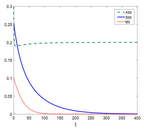
Population dynamics of X(t), S(t) and I(t) of system (1.1) with K=0.2,k=0.01.
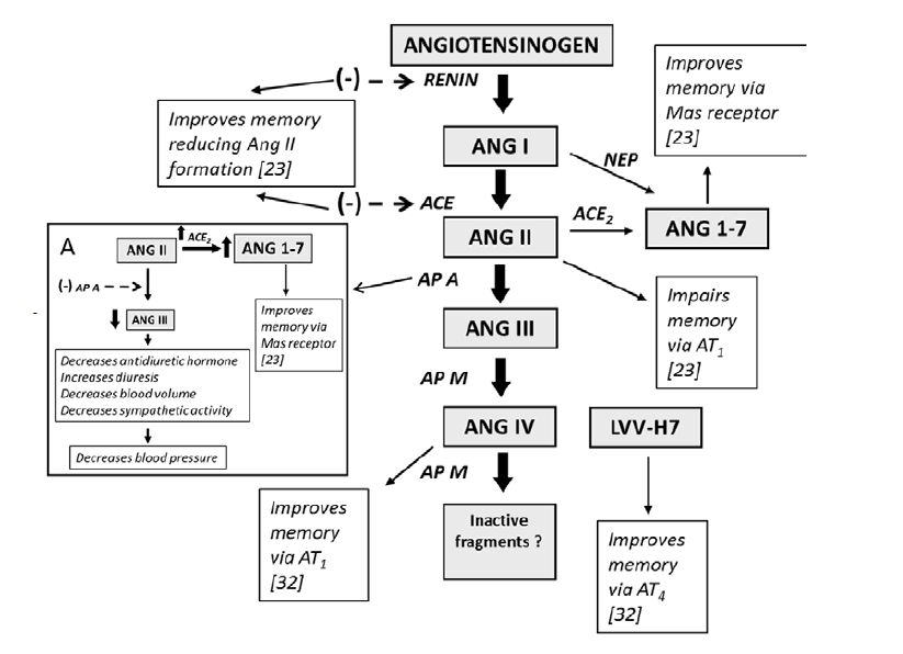
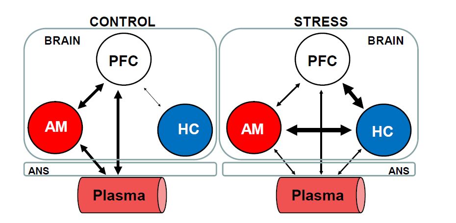
Stress has been demonstrated to be a key modulator in learning and memory processes, in which the hippocampus plays a central role. A great number of neuropeptides have been reported to modulate learning and memory under stressful conditions. Neuropeptidases are proteolytic enzymes capable of regulating the function of neuropeptides in the central and peripheral nervous system. In this regard, a number of neuropeptidases, i.e. angiotensinases, oxytocinase, or enkephalinases, have received attention. Their involvement in stress and memory processes is a promising perspective, as it is possible to influence their activities through various activators or inhibitors and, consequently, to pharmacologically modulate the functions of the endogenous substrates that are involved. The present review describes the key findings showing the involvement of neuropeptides and neuropeptidases in stress and memory and highlights the role of the hippocampus in these processes.
Citation: I. Prieto, A.B. Segarra, M. de Gasparo, M. Ramírez-Sánchez. Neuropeptidases, Stress, and Memory—A Promising Perspective[J]. AIMS Neuroscience, 2016, 3(4): 487-501. doi: 10.3934/Neuroscience.2016.4.487
| [1] | Kawkab Al Amri, Qamar J. A Khan, David Greenhalgh . Combined impact of fear and Allee effect in predator-prey interaction models on their growth. Mathematical Biosciences and Engineering, 2024, 21(10): 7211-7252. doi: 10.3934/mbe.2024319 |
| [2] | Saheb Pal, Nikhil Pal, Sudip Samanta, Joydev Chattopadhyay . Fear effect in prey and hunting cooperation among predators in a Leslie-Gower model. Mathematical Biosciences and Engineering, 2019, 16(5): 5146-5179. doi: 10.3934/mbe.2019258 |
| [3] | Dirk Stiefs, Ezio Venturino, Ulrike Feudel . Evidence of chaos in eco-epidemic models. Mathematical Biosciences and Engineering, 2009, 6(4): 855-871. doi: 10.3934/mbe.2009.6.855 |
| [4] | Yuhong Huo, Gourav Mandal, Lakshmi Narayan Guin, Santabrata Chakravarty, Renji Han . Allee effect-driven complexity in a spatiotemporal predator-prey system with fear factor. Mathematical Biosciences and Engineering, 2023, 20(10): 18820-18860. doi: 10.3934/mbe.2023834 |
| [5] | Yuanfu Shao . Bifurcations of a delayed predator-prey system with fear, refuge for prey and additional food for predator. Mathematical Biosciences and Engineering, 2023, 20(4): 7429-7452. doi: 10.3934/mbe.2023322 |
| [6] | Hongqiuxue Wu, Zhong Li, Mengxin He . Dynamic analysis of a Leslie-Gower predator-prey model with the fear effect and nonlinear harvesting. Mathematical Biosciences and Engineering, 2023, 20(10): 18592-18629. doi: 10.3934/mbe.2023825 |
| [7] | Ranjit Kumar Upadhyay, Swati Mishra . Population dynamic consequences of fearful prey in a spatiotemporal predator-prey system. Mathematical Biosciences and Engineering, 2019, 16(1): 338-372. doi: 10.3934/mbe.2019017 |
| [8] | Shunyi Li . Hopf bifurcation, stability switches and chaos in a prey-predator system with three stage structure and two time delays. Mathematical Biosciences and Engineering, 2019, 16(6): 6934-6961. doi: 10.3934/mbe.2019348 |
| [9] | Rongjie Yu, Hengguo Yu, Chuanjun Dai, Zengling Ma, Qi Wang, Min Zhao . Bifurcation analysis of Leslie-Gower predator-prey system with harvesting and fear effect. Mathematical Biosciences and Engineering, 2023, 20(10): 18267-18300. doi: 10.3934/mbe.2023812 |
| [10] | Wanxiao Xu, Ping Jiang, Hongying Shu, Shanshan Tong . Modeling the fear effect in the predator-prey dynamics with an age structure in the predators. Mathematical Biosciences and Engineering, 2023, 20(7): 12625-12648. doi: 10.3934/mbe.2023562 |
Stress has been demonstrated to be a key modulator in learning and memory processes, in which the hippocampus plays a central role. A great number of neuropeptides have been reported to modulate learning and memory under stressful conditions. Neuropeptidases are proteolytic enzymes capable of regulating the function of neuropeptides in the central and peripheral nervous system. In this regard, a number of neuropeptidases, i.e. angiotensinases, oxytocinase, or enkephalinases, have received attention. Their involvement in stress and memory processes is a promising perspective, as it is possible to influence their activities through various activators or inhibitors and, consequently, to pharmacologically modulate the functions of the endogenous substrates that are involved. The present review describes the key findings showing the involvement of neuropeptides and neuropeptidases in stress and memory and highlights the role of the hippocampus in these processes.
The effect of disease on eco-epidemiology system is a significant topic from both mathematical and ecological perspectives. The disease factor usually leads to a more complex and diverting dynamics than those in the disease-free system [1,2]. Within the interactions between predator and prey, the disease could only spread in prey or predator population, also could spread between prey and predator [3,4,5]. Birds (particularly pelicans) infect vibrio and die by preying on vibrio-infected fish (particularly tilapia) at the Salton Sea in the desert of Southern California [3], which is an example of disease spreads amongst the prey. For the disease in predator, taking fox rabies as an example, foxes (Vulpis) infect rabies and transmit to other foxes or their prey rabbits by biting in Europe and North America [6]. More relevant examples could be found in [7]. From the mathematical epidemiology point of view, one needs much more attention in the dynamics of infected predator to observe whether the presence of the prey allows the survival of a part of the predator population [8].
A variety of diseased predator models have been proposed to study the complex interaction between prey and predator with infected diseases [2,9,10] and the reference therein. Most common epidemic model applied in predator-prey interactions is the SI-type, i.e., the predator population Y(t) is divided into two sub-classes, namely susceptible predator S(t) and infected predator I(t), respectively [10,11,12]. The infection term could be mass-action term (bilinear form) βSI or saturation form βSIS+I [4]. The infected predators usually behave differently with susceptible ones, and suffer an additional death rate. In a epidemic model, the global dynamics are usually determined by the basic reproduction number R0, i.e., the disease will dies out in the population when R0≤1, and the disease will persist in the population when R0>1. However, the basic reproduction number is no longer a threshold parameter determining the global dynamics in diseased predator models, on the contrary, the dynamics are relatively comprehensive and unexpected.
Predation is the key force in a prey-predator interaction, which could affect the size of prey population by direct hunting [9,13,14,15], and elicit a variety of anti-predator responses [16,17,18]. Consequently, prey tends to alter behaviors in a certain extent, such as change of habitat, foraging activity, vigilance, physiological changes. This anti-predator behaviors accelerate the extinction, evolution and development of prey population in the long run. Under the risk of predation, prey may reduce its foraging activity in order to stay alert, leading to starvation which impacts on population growth [19,20]. Therefore, an immediately result of anti-predator behaviors is the reduction of prey growth rate, which is the cost for prey in prey defense [19,21,22,23,24,25,26].
Consider a simple birth-death process of the prey X(t) with the cost of anti-predator behaviors [27]:
| dXdt=[F(k,Y)a]X−dX, |
where X,Y represent the density of the prey and predator, respectively. a is the birth rate of prey, d is the natural death rate of prey. F(k,Y) accounts for the cost of anti-predator defence due to fear, the parameter k reflects the level of fear which drives anti-predator behaviors of prey. The fear factor F(k,Y) has some specific assumptions under the ecological motions, for details see [20,27].
To derive a simple diseased predator model incorporating the anti-predator defence due to fear, we adopted the following fear effect term F(k,Y):
| F(k,Y)=11+kY=11+k(S+I). |
Based on the results in [4,9,11], we can obtain the eco-epidemiological system with cost of anti-predator behaviors as following system of nonlinear differential equations:
| {dXdt=rX1+k(S+I)−rX2K−aXS1+bX,dSdt=eaXS1+bX−d1S−βSI,dIdt=βSI−d2I, | (1.1) |
where X,S,I represent the density of prey, susceptible predator and infected predator at time t, respectively. r is the intrinsic growth rate of prey, K is the carrying capacity of the prey, a is the predation coefficient, b is the predators handling time of a prey, e is the biomass conversion constant, β is the transmissibility coefficient. d1 and d2 are the mortality rates of the susceptible predator and infected predator, and naturally d1<d2.
This paper consists of six sections. In the next section, we prove the positivity and boundedness of the solution of system (1.1). In Section 3, we provide the existence conditions of the equilibria of the model. We analyze the stability of equilibria and show the occurrence of Hopf bifurcation in Section 4. In Section 5, the correctness of the theoretical proof is illustrated by numerical simulation. Finally, we summarize our results with ecological interpretations in Section 6.
In view of the ecological significance, we only consider the solutions (X(t),S(t),I(t)) of system (1.1) on
| R3+={(X(t),S(t),I(t))∈R3+:X(t)≥0,S(t)≥0,I(t)≥0}. |
Theorem 2.1. Each solution of system (1.1) with initial value (X(0),S(0),I(0))∈R3+ is positive and ultimately bounded.
Proof. Since the right-hand side of system (1.1) is completely continuous and locally Lipschitzian on R3+, the solution (X(t),S(t),I(t)) with initial condition (X(0),S(0),I(0))∈R3+ exists and is unique on R3+.
By integrating, it follows from system (1.1) that
| X(t)=X(0)exp{t∫0(r1+k(S(τ)+I(τ))−rX(τ)K−aS(τ)1+bX(τ))dτ}≥0,S(t)=S(0)exp{t∫0(eaX(τ)1+bX(τ)−d1−βI(τ))dτ}≥0,I(t)=I(0)exp{t∫0(βS(τ)−d2)dτ}≥0. |
Hence, the solution (X(t),S(t),I(t)) of system (1.1) with the initial condition (X(0),S(0),I(0))∈R3+ remains positive.
From the first equation of (1.1), we can obtain
| dXdt=rX1+k(S+I)−rX2K−aXS1+bX≤rX−rX2K=rX(1−XK), |
then
| lim supt→∞X(t)≤K. |
Let N(t)=eX(t)+S(t)+I(t), we can get
| dNdt=erX1+k(S+I)−erX2K−d1S−d2I≤erX−erX2K−d1S−d2I≤erX(1−XK)+ed1X−d1N≤eK(r+d1)24r−d1N, |
then
| lim supt→∞N(t)≤eK(r+d1)24rd1. |
This ends the proof.
Remark 2.2. From Theorem 2.1, we know that all positive solutions of system (1.1) with initial conditions (X(0),S(0),I(0))∈R3+ are defined in the following positive bounded invariant:
| Γ:={(X(t),S(t),I(t))∈R3+:0≤X(t)≤K,0≤eX(t)+S(t)+I(t)≤eK(r+d1)24rd1}. |
System (1.1) possesses at most three boundary equilibria:
(i) Trivial equilibrium: E0=(0,0,0);
(ii) Axial equilibrium: E1=(K,0,0);
(iii) Planar equilibrium: E2=(X2,S2,0) exists if ea−bd1>0 and K>d1ea−bd1, where
| X2=d1ea−bd1,S2=−[K(ea−bd1)2+rd1ke]+√[K(ea−bd1)2−rd1ke]2+4K2kre(ea−bd1)32Kk(ea−bd1)2. | (3.1) |
For epidemic models, the most critical problem is the threshold property for the extinction and persistence of the disease, which is generally governed by the basic reproduction number R0. The basic reproduction number can be interpreted as the expected number of secondary cases produced, in a completely susceptible population, by a typical infected individual during its entire period of infectiousness. Following [28], we define the basic reproduction number for the predator population in the system (1.1) by
| R0:=βS2d2, |
where S2 is given by (3.1).
Next, we mainly focus on the existence of positive equilibrium E3=(X3,S3,I3) of system (1.1). The coordinates X3,S3,I3 are positive solutions to the following system of equilibrium equations:
| {r1+k(S3+I3)−rX3K−aS31+bX3=0,eaX31+bX3−d1−βI3=0,βS3−d2=0. |
Thus,
| S3=d2β,I3=X3(ea−bd1)−d1(bX3+1)β, |
and X3 is the positive root of (3.2) in (X2,+∞):
| Q(X)=m3X3+m2X2+m1X+m0=0, | (3.2) |
where
| m3:=−bβr(k(ea−bd1)+b(kd2+β)),m2:=βr(Kb2β−k(ea−bd1)−2b(kd2+β)+bkd1),m1:=(−kd2a(ea−bd1)−b(akd22+aβd2−2β2r))K−βr(−kd1+kd2+β),m0:=−K(−ad2(kd1−kd2−β)−β2r). |
If ea−bd1>0 and r>ad2(β+k(d2−d1))β2, we have
| m3<0,m0>0. |
By Descartes' rule of signs, system (1.1) has at least one positive equilibrium E3.
Hence, we have the following results on the existence of the positive equilibrium. It is worthy to note that the positive equilibrium is not unique due to the impact of fear effect k.
Theorem 3.1. If ea−bd1>0 and r>ad2(β+k(d2−d1))β2, then system (1.1) has at least one positive equilibrium E3=(X3,S3,I3), where S3=S2R0, I3=X3(ea−bd1)−d1(bX3+1)β and X3 is the positive root of (3.2) in (X2,+∞).
Regarding the local stability of trivial equilibrium E0 and axial equilibrium E1, we have the following results. The proof is standard, so we omit it here.
Theorem 4.1. For system (1.1),
(i) The trivial equilibrium E0=(0,0,0) is unstable;
(ii) If one of the following inequalities holds:
(ii-1) ea−bd1<0;
(ii-2) ea−bd1>0 and K<d1ea−bd1,
then the axial equilibrium E1=(K,0,0) is stable; while E1=(K,0,0) is unstable if ea−bd1>0 and K>d1ea−bd1.
Secondly, we will show the local stability of the planar equilibrium E2 of system (1.1). For convenience, set
| r1:=d2(ea−bd1)βe,r2:=d2(ea−bd1)(ea+bd1)aβe2,K1:=ea+bd1b(ea−bd1),K2:=βerd1(ea−bd1)(βer−d2(ea−bd1)),k1:=Kb(ea−bd1)2(Kb(ea−bd1)−(ea+bd1))ae2r(ea+bd1),k2:=−β((ea−bd1)(d2(ea−bd1)−βer)K+βerd1)(Kd2(ea−bd1)2+βerd1)d2. | (4.1) |
Theorem 4.2. For system (1.1), assume that ea−bd1>0. If one of the following inequalities holds:
(Ⅰ) r≤r1 and one of the following inequalities holds:
(Ⅰ-1) d1ea−bd1<K≤K1;
(Ⅰ-2) K>K1 and k>k1;
(Ⅱ) r1<r<r2 and one of the following inequalities holds:
(Ⅱ-1) d1ea−bd1<K≤K1;
(Ⅱ-2) K1<K and k>max{k1,k2};
(Ⅲ) r>r2 and one of the following inequalities holds:
(Ⅲ-1) d1ea−bd1<K≤K2;
(Ⅲ-2) K2<K and k>max{k1,k2},
then equilibrium E2 is stable; otherwise, it is unstable.
Proof. The Jacobian matrix of system (1.1) at E2 is given by
| J2=(a11a12a13a210−βS200βS2−d2), |
where
| a11:=X2(−rK+abS2(1+bX2)2),a12:=−krX2(1+kS2)2−aX21+bX2,a13:=−krX2(1+kS2)2,a21:=eaS2(1+bX2)2. |
Hence, the characteristic equation of J2 is given as
| f(λ)(λ−βS2+d2)=0, | (4.2) |
where
| f(λ):=λ2−a11λ−a12a21. |
Clearly, one can see that J2 has three eigenvalues λ1, λ2 and λ3=βS2−d2. Since a12<0,a21>0, then −a12a21>0.
From (3.1), we can obtain
| a11=X2(−rK+abS2(1+bX2)2)=X2Φ2Kka2e2, |
where
| Φ:=ab√(K(ea−bd1)2−rd1ke)2+4K2kre(ea−bd1)3−ab(K(ea−bd1)2+rd1ke)−2rka2e2. |
Note that the sign of Φ depends on
| ˜Φ:=a2b2((K(ea−bd1)2−rd1ke)2+4K2kre(ea−bd1)3)−(ab(K(ae−bd1)2+rd1ke)+2rka2e2)2=4a2kerP(k), |
where
| P(k):=−ae2r(ea+bd1)k+Kb(ea−bd1)2(Kb(ea−bd1)−(ea+bd1)). |
One can obtain that P(k) is decreasing with respect to k. If K≤ea+bd1b(ea−bd1) holds, we have P(0)≤0, which means that P(k)<0 for all k>0; if K>ea+bd1b(ea−bd1) and k>k1 hold, we can get P(k)<0. Therefore, when one of the following inequalities holds:
(i) K≤ea+bd1b(ea−bd1);
(ii) K>ea+bd1b(ea−bd1) and k>k1,
we can obtain a11<0, which implies that the real parts of λ1 and λ2 are all negative.
It follows from system (3.1) that
| βS2−d2=−β[K(ea−bd1)2+rd1ke]+β√[K(ea−bd1)2−rd1ke]2+4K2kre(ea−bd1)32Kk(ea−bd1)2−d2=Θ2Kk(ea−bd1)2, |
where
| Θ:=−K(ea−bd1)2(2kd2+β)−βekrd1+β√(K(ea−bd1)2−rd1ke)2+4K2kre(ea−bd1)3. |
Note that the sign of Θ depends on
| ˜Θ:=β2(K(ea−bd1)2−rd1ke)2+4β2K2kre(ea−bd1)3−(K(ea−bd1)2(2kd2+β)+βekrd1)2=−4Kk(ae−bd1)2[(Kd2(ea−bd1)2+βerd1)d2k+β((ea−bd1)(d2(ea−bd1)−βer)K+βerd1)]. |
Then if one of the following inequalities holds:
(Ⅰ) ea−bd1>0 and r≤d2(ea−bd1)βe;
(Ⅱ) ea−bd1>0, r>d2(ea−bd1)βe and one of the following inequalities:
(Ⅱ-1) K≤βerd1(ea−bd1)(βer−d2(ea−bd1));
(Ⅱ-2) K>βerd1(ea−bd1)(βer−d2(ea−bd1)) and k>k2:=−β((ea−bd1)(d2(ea−bd1)−βer)K+βerd1)(Kd2(ea−bd1)2+βerd1)d2,
we have λ3=βS2−d2<0.
Thus, we can arrive at the conclusion.
It should be pointed out that another way to state Theorem 4.2 is as follows.
Remark 4.3. For system (1.1), assume that ea−bd1>0 and R0<1. If one of the following inequalities:
(Ⅰ) d1ea−bd1<K≤K1;
(Ⅱ) K>K1 and k>k1
holds, then the planar equilibrium E2 is stable; otherwise, it is unstable.
Next, we will show the local stability of the positive equilibrium E3 of system (1.1).
The Jacobian matrix of system (1.1) at E3 is given by
| J3=(b11b12b13b210−d20βI30), |
where
| b11=X3(−rK+abS3(1+bX3)2),b12=−krX3(1+k(S3+I3))2−aX31+bX3<0,b13=−krX3(1+k(S3+I3))2<0,b21=eaS3(1+bX3)2>0. | (4.3) |
The characteristic equation of J3 is given as
| λ3+A1λ2+A2λ+A3=0, | (4.4) |
where
| A1=−b11,A2=βd2I3−b12b21,A3=−b11βd2I3−b13b21βI3. | (4.5) |
Note that if A1>0 holds, then b11<0, which means that A3>0. According to Routh-Hurwitz criterion, the positive equilibrium E3 is locally asymptotically stable when A1>0 and A1A2−A3>0.
Therefore, we can establish the following statement.
Theorem 4.4. Assume that ea−bd1>0 and r>ad2(β+k(d2−d1))β2 hold. The positive equilibrium E3 of system (1.1) is locally asymptotically stable if A1>0 and A1A2−A3>0, where Ai,i=1,2,3 is defined as in (4.5). Otherwise, it is unstable.
Remark 4.5. Theorem 4.4 gives a sufficient condition about the stability of the positive equilibrium E3 for system (1.1). However, the complexity of model (1.1) leads to the failure to theoretically demonstrate how the fear factor affects the stability of the positive equilibrium. This will be discussed later through numerical simulations.
In this subsection, we take k as the bifurcation parameter. The characteristic equation of system (1.1) at E3 is (4.4), and Ai(k),i=1,2,3 are defined as (4.5).
Theorem 4.6. Hopf bifurcation near the positive equilibrium E3 for system (1.1) occurs whenever the critical parameter k attains the value k=kh in the domain:
| Ω={kh∈R+:Δ(kh):=[A1(k)A2(k)−A3(k)]|k=kh=0withA2(kh)>0,[dΔ(k)dk]|k=kh≠0}. |
Proof. If k=kh, the characteristic Eq (4.4) equals
| λ3+A1(kh)λ2+A2(kh)λ+A3(kh)=0, | (4.6) |
then (4.6) can be factorized as
| (λ2+A2(kh))(λ+A1(kh))=0. | (4.7) |
Clearly, (4.7) has three roots: λ1=i√A2(kh), λ2=−i√A2(kh) and λ3=−A1(kh). The roots are of the form λ1=p1(k)+ip2(k), λ2=p1(k)−ip2(k) and λ3=−p3(k), where pi(k)(i=1,2,3) are real numbers.
From the characteristic Eq (4.4), we can get
| dλdk=−λ2A′1+λA′2+A′33λ2+2A1λ+A2, | (4.8) |
where ′=ddk. Substituting λ=i√A2 into (4.8), we obtain that
| A′3−A2A′1+iA′2√A22(A2−iA1√A2)=−dΔ(k)dk2(A21+A2)+i[√A2A′22A2−A1√A2dΔ(k)dk2A2(A21+A2)], |
which implies that
| [dRe(λ)dk]|k=kh=−dΔ(k)dk2(A21+A2)|k=kh. |
By using monotonicity condition in the real part of the complex root dRe(λ)dk|k=kh≠0, the transversality condition dΔ(k)dk|k=kh≠0 can be obtained to ensure the existence of Hopf bifurcation.
Results from numerical simulations are provided in this section to demonstrate our theoretical results. As we will show, the observations shed lights on the impact of fear factor. We choose the parameters of system (1.1) as follows:
| r=0.8,a=0.2,b=0.1,e=0.9,d1=0.05,β=0.1,d2=0.053. | (5.1) |
Then we have
| ea−bd1=0.175>0,d1ea−bd1=0.286,r1=d2(ea−bd1)βe=0.103,r2=d2(ea−bd1)(ea+bd1)aβe2=0.106,K1=ea+bd1b(ea−bd1)=10.571,K2=βerd1(ea−bd1)(βer−d2(ea−bd1))=0.328. |
Example 5.1 (The stability of E1).
We adopt K=0.2,k=0.01, then system (1.1) has trivial equilibrium E0=(0,0,0) and axial equilibrium E1=(0.2,0,0). In this case, one can know that the conditions of Theorem 4.1 are satisfied, which means that E1 is locally asymptotically stable. The numerical results are shown in Figure 1.
Example 5.2 (The impacts of K and k on the stability of E2).
In this example, we will choose three values of carrying capacity K for numerical experiments. We conclude that the carrying capacity and fear effect are other key factors related to the extinction of infected predators, in addition to the basic reproduction number R0.
Firstly, we take K=0.3<K2, then we have k=0.1 which yields that R0=0.263<1. In this case, system (1.1) has trivial equilibrium E0=(0,0,0), axial equilibrium E1=(0.3,0,0), and planar equilibrium E2=(0.286,0.139,0). By Theorem 4.5, E2 is locally asymptotically stable, see Figure 2(a). Thus, when the carrying capacity of the prey K is small, no matter what the level of fear k is, the small size of prey population will lead to the extinction of infected predators.

Secondly, for comparison, we take K2<K=15, then
| k1=Kb(ea−bd1)2(Kb(ea−bd1)−(ea+bd1))ae2r(ea+bd1)=0.149,k2=−β((ea−bd1)(d2(ea−bd1)−βer)K+βerd1)(Kd2(ea−bd1)2+βerd1)d2=10.873. |
Choosing k=0.1<max{k1,k2} which yields R0=5.792>1, then we have
| A1=0.25791>0,A1A2−A3=0.00523>0. |
In this case, system (1.1) has trivial equilibrium E0=(0,0,0), axial equilibrium E1=(15,0,0), planar equilibrium E2=(0.286,3.070,0), and positive equilibrium E3=(7.351,0.530,7.125). By Theorem 4.5, E2=(0.286,3.070,0) is unstable. On the contrary, E3=(7.351,0.530,7.125) is locally asymptotically stable. The numerical simulation is shown in Figure 2(b).
Finally, we take K2<K=60, then we have
| k1=Kb(ea−bd1)2(Kb(ea−bd1)−(ea+bd1))ae2r(ea+bd1)=6.629,k2=−β((ea−bd1)(d2(ea−bd1)−βer)K+βerd1)(Kd2(ea−bd1)2+βerd1)d2=12.238. |
Choosing k=30>max{k1,k2} which yields that R0=0.649<1, system (1.1) has trivial equilibrium E0=(0,0,0), axial equilibrium E1=(60,0,0), and planar equilibrium E2=(0.286,0.344,0). By Theorem 4.5, E2 is locally asymptotically stable, see Figure 2(c). Thus, when the carrying capacity of the prey K is relatively large, a high level of fear k will lead to the extinction of infected predators.
Example 5.3 (The impact of k on the stability of E3). We adopt K=60, then we have kh=0.26. In the next, we will choose three values of k, corresponding to the local stability of E3, Hopf bifurcation, and instability of E3, to illustrate the impact of fear factor on the population dynamics.
Firstly, we take k=0.1<kh which yields that R0=5.881>1, then system (1.1) has trivial equilibrium E0=(0,0,0), axial equilibrium E1=(60,0,0), planar equilibrium E2=(0.286,3.117,0) and a unique positive equilibrium E3=(24.047,0.530,12.213). In this case, we obtain that
| A1=0.29863>0,A1A2−A3=0.00065>0, |
which means that E3 is local asymptotically stable. The numerical results are shown in Figure 3.

Secondly, we take k=0.26=kh which yields that R0=4.682>1, then system (1.1) has trivial equilibrium E0=(0,0,0), axial equilibrium E1=(60,0,0), planar equilibrium E2=(0.286,2.481,0) and a unique positive equilibrium E3=(12.975,0.530,9.665). In this case, we obtain that
| A1=0.14694>0,A1A2−A3=0, |
which means that system (1.1) undergoes a Hopf bifurcation and there is a limit cycle around E3. The numerical results and the bifurcation diagrams of system (1.1) with respect to the parameter k are shown in Figures 4 and 5, respectively. Comparing Figures 3 and 4(a), one can see that there are two different implications induced by the fear factor k: the first is that the stability of E3 converts from stable into unstable, and the second is the decrease of values of X3 and I3 of E3.


Finally, we take k=0.5>kh which yields that R0=3.821>1, then system (1.1) has trivial equilibrium E0=(0,0,0), axial equilibrium E1=(60,0,0), planar equilibrium E2=(0.286,2.025,0) and a unique positive equilibrium E3=(7.685,0.530,7.322). In this case, we can obtain that
| A1=0.07642>0,A1A2−A3=−0.00051<0, |
which means that E3 is unstable. The numerical results are shown in Figure 6. One can find that the difference between Figures 4 and 6 is the decrease of values of E3 from (12.975,0.530,9.665) to (7.685,0.530,7.322), which is induced by the impact of the feat factor.

In this paper, we explored a predator-prey model that incorporates infectious disease in predator population and the cost of anti-predator behaviors. The cost of anti-predator behaviors is measured by a fear effect k leading to an reduction of prey's birth rate. We fulfill a complete stability analysis of equilibria for system (1.1) and show that the system (1.1) exhibits the Hopf bifurcation. Biologically, we focus on the impact of fear effect on the population dynamics. As we will see later, the cost of a high level of fear effect is disastrously. The main findings are summarized in the following.
1) Small size of prey population leads to the extinction of infected predators.
If the carrying capacity K is relatively small, the planar equilibrium E2 is stable, see Figure 2(a). Thus, no matter what the level of fear effect k is, a small size of prey population will lead to the extinction of infected predators.
2) Low level of the fear effect doesn't impact on the population dynamics.
If the level of fear effect k<kh, the positive (coexistence) equilibrium E3 is stable, see Figure 3. Hence, we conclude that a small fear effect k is not the key disturbance and does not change the coexistence dynamics of system (1.1). However, the densities of the prey and infected predator gradually decrease as k increasing.
3) Certain medium level of the fear effect lead to periodic oscillation.
If k=kh, the fear effect can destabilize the stability of E3 and will benefit the occurrence of periodic oscillation. In other words, system (1.1)undergoes a limit cycle, see Figures 4 and 5.
4) High level of the fear effect leads to complex dynamics and the infected predator can go to extinction.
If k>kh, E3 is unstable, see Figure 6. Therefore, a large fear effect k persistently and dramatically influence the population dynamics of prey and predator. Furthermore, if the level of the fear factor k is extremely high, the planar equilibrium E2 is stable, see Figure 2(c). The prey will respond to perceived predation risk and show a variety of anti-predator responses, dramatically decreasing the recruitment of susceptible predator, which will lead to an extinction of infected predator.
The authors would like to thank the editor and the referees for their helpful comments. This research was supported by the National Natural Science Foundation of China (Grant No. 12171192, 12031020 and 12071173), the Science and Technology Research Projects of the Education Office of Jilin Province, China (JJKH20211033KJ), the Technology Development Program of Jilin Province, China (20210508024RQ) and Huaian Key Laboratory for Infectious Diseases Control and Prevention, China (HAP201704).
The authors declare that there are no conflicts of interest regarding the publication of this paper.
| [1] |
Goldstein DS, Kopin IJ (2007) Evolution of concepts of stress. Stress 10: 109-120. doi: 10.1080/10253890701288935

|
| [2] | Sterling P (2012) Allostasis: a model of predictive regulation. Physiol Behav 106: 5-15. |
| [3] |
Davidson RJ, McEwen BS (2012) Social influences on neuroplasticity: stress and interventions to promote well-being. Nat Neurosci 15: 689-695. doi: 10.1038/nn.3093
|
| [4] |
Godsil BP, Kiss JP, Spedding M, et al. (2013) The hippocampal-prefrontal pathway: the weak link in psychiatric disorders? Eur Neuropsychopharmacol 23: 1165-1181. doi: 10.1016/j.euroneuro.2012.10.018
|
| [5] |
McEwen BS (2007) Physiology and neurobiology of stress and adaptation: central role of the brain. Physiol Rev 87: 873-904. doi: 10.1152/physrev.00041.2006
|
| [6] |
Ulrich-Lai YM, Herman JP (2009) Neural regulation of endocrine and autonomic stress responses. Nat Rev Neurosci 10: 397-409. doi: 10.1038/nrn2647
|
| [7] |
Hernández J, Prieto I, Segarra AB, et al. (2015) Interaction of neuropeptidase activities in cortico-limbic regions after acute restraint stress. Behav Brain Res 287: 42-48. doi: 10.1016/j.bbr.2015.03.036
|
| [8] | Segarra AB, Hernández J, Prieto I, et al. (2016) Neuropeptidase activities in plasma after acute restraint stress. Interaction with cortico-limbic areas. Acta Neuropsychiatr 28: 239-243. |
| [9] | Sandi C, Pinelo-Nava MT (2007) Stress and memory: behavioral effects and neurobiological mechanisms. Neural Plast 2007: 78970. |
| [10] |
Schwabe L, Joëls M, Roozendaal B, et al. (2012) Stress effects on memory: an update and integration. Neurosci Biobehav Rev 36: 1740-1749. doi: 10.1016/j.neubiorev.2011.07.002
|
| [11] |
Richter-Levin G, Akirav I (2000) Amygdala-hippocampus dynamic interaction in relation to memory. Mol Neurobiol 22: 11-20. doi: 10.1385/MN:22:1-3:011
|
| [12] | Kim JJ, Diamond DM (2002) The stressed hippocampus, synaptic plasticity and lost memories. Nat Rev Neurosci 3: 453-462. |
| [13] |
Sebastian V, Estil JB, Chen D, et al. (2013) Acute physiological stress promotes clustering of synaptic markers and alters spine morphology in the hippocampus. PLoS One 8: e79077. doi: 10.1371/journal.pone.0079077
|
| [14] |
Moss RA (2016) A Theory on the Singular Function of the Hippocampus: Facilitating the Binding of New Circuits of Cortical Columns. AIMS Neurosci 3: 264-305. doi: 10.3934/Neuroscience.2016.3.264
|
| [15] |
Toth I, Neumann ID (2013) Animal models of social avoidance and social fear. Cell Tissue Res 354: 107-118. doi: 10.1007/s00441-013-1636-4
|
| [16] |
Campos AC, Fogaça MV, Aguiar DC, et al. (2013) Animal models of anxiety disorders and stress. Rev Bras Psiquiatr 35: S101-111. doi: 10.1590/1516-4446-2013-1139
|
| [17] | Sandi C, Pinelo-Nava MT (2007) Stress and memory: behavioral effects and neurobiological mechanisms. Neural Plast 2007: 78970. |
| [18] |
Gülpinar MA, Yegen BC (2004) The physiology of learning and memory: role of peptides and stress. Curr Protein Pept Sci 5: 457-473. doi: 10.2174/1389203043379341
|
| [19] | Bilkei-Gorzo A, Racz I, Michel K, et al. (2008) Control of hormonal stress reactivity by the endogenous opioid system. Psychoneuroendocrinology 33: 425-436. |
| [20] | Narita M, Kaneko C, Miyoshi K, et al. (2006) Chronic pain induces anxiety with concomitant changes in opioidergic function in the amygdala. Neuropsychopharmacology 3:739-750. |
| [21] | Neumann ID, Torner L, Wigger A (2000) Brain oxytocin: differential inhibition of neuroendocrine stress responses and anxiety-related behaviour in virgin, pregnant and lactating rats. Neuroscience 95: 567-575. |
| [22] |
Neumann ID (2007) Stimuli and consequences of dendritic release of oxytocin within the brain. Bioch Soc Trans 35: 1252-1257. doi: 10.1042/BST0351252
|
| [23] |
Wright JW, Yamamoto BJ, Harding JW (2008) Angiotensin receptor subtype mediated physiologies and behaviors: new discoveries and clinical targets. Prog Neurobiol 84: 157-181. doi: 10.1016/j.pneurobio.2007.10.009
|
| [24] |
Saavedra JM, Benicky J (2007) Brain and peripheral angiotensin II play a major role in stress. Stress 10: 185-193. doi: 10.1080/10253890701350735
|
| [25] | Nomura S, Ito T, Mizutani S (2004) Placental leucine aminopeptidase. Aminopeptidases in biology and disease. Kluwer Academic/Plenum, New York, Hooper NM and Lendeckel U Eds. pp 45-59. |
| [26] |
Solhonne B, Gros C, Pollard H, et al. (1987) Major localization of aminopeptidase M in rat brain. Neuroscience 22: 225-232. doi: 10.1016/0306-4522(87)90212-0
|
| [27] | Thompson MW, Hersh LB (2004) The puromycin-sensitive aminopeptidase. Aminopeptidases in biology and disease. Kluwer Academic/Plenum, New York, Hooper NM and Lendeckel U Eds. pp 1-15. |
| [28] |
Ramírez-Sánchez M, Prieto I, Wangensteen R, et al. (2013) The renin-angiotensin system: new insight into old therapies. Curr Med Chem 20: 1313-1322. doi: 10.2174/0929867311320100008
|
| [29] | Prieto I, Villarejo AB, Segarra AB, et al. (2015) Tissue distribution of CysAP activity and its relationship to blood pressure and water balance. Life Sci 134: 173-178. |
| [30] |
Albiston AL, Mustafa T, McDowall SG, et al. (2003) AT4 receptor is insulin-regulated membrane aminopeptidase: potential mechanisms of memory enhancement. Trends Endocrinol Metab 14: 72-77. doi: 10.1016/S1043-2760(02)00037-1
|
| [31] |
De Bundel D, Smolders I,Vanderheyden P, et al. (2008) Ang II and Ang IV: unraveling the mechanism of action on synaptic plasticity, memory, and epilepsy. CNS Neurosci Ther 14: 315-339. doi: 10.1111/j.1755-5949.2008.00057.x
|
| [32] |
De Bundel D, Demaegdt H, Lahoutte T, et al. (2010) Involvement of the AT1 receptor subtype in the effects of angiotensin IV and LVV-haemorphin 7 on hippocampal neurotransmitter levels and spatial working memory. J Neurochem 112: 1223-1234. doi: 10.1111/j.1471-4159.2009.06547.x
|
| [33] |
Drolet G, Dumont EC, Gosselin I, et al. (2001) Role of endogenous opioid system in the regulation of the stress response. Prog Neuropsychopharmacol Biol Psychiatry 25: 729-741. doi: 10.1016/S0278-5846(01)00161-0
|
| [34] |
McCubbin JA (1993) Stress and endogenous opioids: behavioral and circulatory interactions. Biol Psychol 35: 91-122. doi: 10.1016/0301-0511(93)90008-V
|
| [35] |
Bodnar RJ (2014) Endogenous opiates and behavior: 2013. Peptides 62: 67-136. doi: 10.1016/j.peptides.2014.09.013
|
| [36] |
Bodnar RJ (2016) Endogenous opiates and behavior: 2014. Peptides 75: 18-70. doi: 10.1016/j.peptides.2015.10.009
|
| [37] | Bali A, Randhawa PK, Jaggi AS (2015) Stress and opioids: role of opioids in modulating |
| [38] | stress-related behavior and effect of stress on morphine conditioned place preference. Neurosci Biobehav Rev 51: 1150. |
| [39] |
38. Olff M, Frijling JL, Kubzansky LD, et al. (2013) The role of oxytocin in social bonding, stress regulation and mental health: an update on the moderating effects of context and interindividual differences. Psychoneuroendocrinology 38: 1883-1894. doi: 10.1016/j.psyneuen.2013.06.019
|
| [40] |
39. Okimoto N, Bosch OJ, Slattery DA, et al. (2012) RGS2 mediates the anxiolytic effect of oxytocin. Brain Res 1453: 26-33. doi: 10.1016/j.brainres.2012.03.012
|
| [41] |
40. Neumann ID, Slattery DA (2016) Oxytocin in General Anxiety and Social Fear: A Translational Approach. Biol Psychiatry 79: 213-221. doi: 10.1016/j.biopsych.2015.06.004
|
| [42] |
41. Light KC, Grewen KM, Amico JA, et al. (2004) Deficits in plasma oxytocin responses and increased negative affect, stress, and blood pressure in mothers with cocaine exposure during pregnancy. Addict Behav 29: 1541-1564. doi: 10.1016/j.addbeh.2004.02.062
|
| [43] |
42. Linnen AM, Ellenbogen MA, Cardoso C, et al. (2012) Intranasal oxytocin and salivary cortisol concentrations during social rejection in university students. Stress 15: 393-402. doi: 10.3109/10253890.2011.631154
|
| [44] |
43. Norman GJ, Cacioppo JT, Morris JS, et al. (2011) Oxytocin increases autonomic cardiac control: moderation by loneliness. Biol Psychol 86: 174-180. doi: 10.1016/j.biopsycho.2010.11.006
|
| [45] |
44. Windle RJ, Kershaw YM, Shanks N, et al. (2004) Oxytocin attenuates stress-induced c-fos mRNA expression in specific forebrain regions associated with modulation of hypothalamo-pituitary-adrenal activity. J Neurosci 24: 2974-2982. doi: 10.1523/JNEUROSCI.3432-03.2004
|
| [46] |
45. Domes G, Heinrichs M, Gläscher J, et al. (2007) Oxytocin attenuates amygdala responses to emotional faces regardless of valence. Biol Psychiatry 62: 1187-1190. doi: 10.1016/j.biopsych.2007.03.025
|
| [47] |
46. Kirsch P, Esslinger C, Chen Q, et al. (2005) Oxytocin modulates neural circuitry for social cognition and fear in humans. J Neurosci 25: 11489-11493. doi: 10.1523/JNEUROSCI.3984-05.2005
|
| [48] |
47. Viviani D, Charlet A, van den Burg E, et al. (2011) Oxytocin selectively gates fear responses through distinct outputs from the central amygdala. Science 333: 104-107. doi: 10.1126/science.1201043
|
| [49] |
48. Sripada CS, Phan KL, Labuschagne I, et al. (2013) Oxytocin enhances resting-state connectivity between amygdala and medial frontal cortex. Int J Neuropsychopharmacol 16: 255-260. doi: 10.1017/S1461145712000533
|
| [50] |
49. Ferguson JN, Young LJ, Hearn EF, et al. (2000) Social amnesia in mice lacking the oxytocin gene. Nat Genet 25: 284-288. doi: 10.1038/77040
|
| [51] |
50. Wirth MM (2015) Hormones, stress, and cognition: The effects of glucocorticoids and oxytocin on memory. Adapt Human Behav Physiol 1: 177-201. doi: 10.1007/s40750-014-0010-4
|
| [52] | 51. McDonald JK, Barrett AJ (1986) Mammalian proteases: a glossary and bibliography (Academic Press, London) vol 2. |
| [53] | 52. Checler F (1993) Methods in neurotransmitter and neuropeptide research, eds Parvez SH, Naoi M, Nagatsu T, Parvez S (Elsevier, Amsterdam). |
| [54] |
53. Ramírez M, Prieto I, Banegas I, et al. (2011) Neuropeptidases. Methods Mol Biol 789: 287-294. doi: 10.1007/978-1-61779-310-3_18
|
| [55] |
54. Morales-Mulia M, de Gortari P, Amaya MI, et al. (2012) Activity and expression of enkephalinase and aminopeptidase N in regions of the mesocorticolimbic system are selectively modified by acute ethanol administration. J Mol Neurosci 46: 58-67. doi: 10.1007/s12031-011-9623-2
|
| [56] |
55. Ramírez M, Prieto I, Alba F, et al. (2008) Role of central and peripheral aminopeptidase activities in the control of blood pressure: a working hypothesis. Heart Fail Rev 13: 339-353. doi: 10.1007/s10741-007-9066-6
|
| [57] |
56. Reid KJ, McGee-Koch LL, Zee PC (2011) Cognition in circadian rhythm sleep disorders. Prog Brain Res 190: 3-20. doi: 10.1016/B978-0-444-53817-8.00001-3
|
| [58] | 57. Wright KP, Lowry CA, Lebourgeois MK (2012) Circadian and wakefulness-sleep modulation of cognition in humans. Front Mol Neurosci 5: 50. |
| [59] |
58. Ramírez M, Prieto I, Vives F, et al. (2004) Neuropeptides, neuropeptidases and brain asymmetry. Curr Protein Pept Sci 5: 497-506. doi: 10.2174/1389203043379350
|
| [60] | 59. Turner AJ (2004) Neprilysin, In Handbook of Proteolytic Enzymes, eds Barrett AJ, Rawlings ND, Woessner JF (Elsevier, London) 419-426. |
| [61] |
60. Iwata N, Takaki Y, Fukami S, et al. (2002) Region-specific reduction of A beta-degrading endopeptidase, neprilysin, in mouse hippocampus upon aging. J Neurosci Res 70: 493-500. doi: 10.1002/jnr.10390
|
| [62] |
61. Iwata N, Mizukami H, Shirotani K, et al. (2004) Presynaptic localization of neprilysin contributes to efficient clearance of amyloid-beta peptide in mouse brain. J Neurosci 24: 991-998. doi: 10.1523/JNEUROSCI.4792-03.2004
|
| [63] |
62. Li L, Tang BL (2005) Environmental enrichment and neurodegenerative diseases. Biochem Biophys Res Commun 334: 293-297. doi: 10.1016/j.bbrc.2005.05.162
|
| [64] |
63. Deweerdt S (2011) Prevention: activity is the best medicine. Nature 475: S16-17. doi: 10.1038/475S16a
|
| [65] |
64. Albiston AL, Fernando R, Ye S, et al. (2004) Alzheimer's, angiotensin IV and an aminopeptidase. Biol Pharm Bull 27: 7767. doi: 10.1248/bpb.27.765
|
| [66] |
65. Marvar PJ, Goodman J, Fuchs S, et al. (2014) Angiotensin type 1 receptor inhibition enhances the extinction of fear memory. Biol Psychiatry 75: 864-872. doi: 10.1016/j.biopsych.2013.08.024
|
| [67] | 66. Hmazzou R, Flahault A, Marc Y, et al. (2016) [OP.6D.03] Mode of action of rb150, an aminopeptidase a inhibitor prodrug as a centrally-acting antihypertensive agent in doca-salt hypertensive rats. J Hypertens 34 Suppl 2: e75. |
| [68] |
67. Hernández J, Segarra AB, Ramírez M, et al. (2009) Stress influences brain enkephalinase, oxytocinase and angiotensinase activities: a new hypothesis. Neuropsychobiology 59: 184-189. doi: 10.1159/000219306
|
| [69] |
68. Tuppy H, Nesbadva H (1957) The aminopeptidase acitvity of serum in pregnancy and its relationship to the potential for inactivating oxytocin. Monatsh Chem 88: 977-988. doi: 10.1007/BF00905420
|
| [70] |
69. Tsujimoto M, Mizutani S, Adachi H, et al. (1992) Identification of human placental leucine aminopeptidase as oxytocinase. Arch Biochem Biophys 292: 388-392. doi: 10.1016/0003-9861(92)90007-J
|
| [71] |
70. Keller SR (2003) The insulin-regulated aminopeptidase: a companion and regulator of GLUT4. Front Biosci 8: s410-420. doi: 10.2741/1078
|
| [72] |
71. Stragier B, De Bundel D, Sarre S, et al. (2008) Involvement of insulin-regulated aminopeptidase in the effects of the renin-angiotensin fragment angiotensin IV: a review. Heart Fail Rev 13: 321-337. doi: 10.1007/s10741-007-9062-x
|
| [73] | 72. Gard PR (2008) Cognitive-enhancing effects of angiotensin IV. BMC Neurosci 9 Suppl 2: S15. |
| [74] |
73. Banegas I, Prieto I, Vives F, et al. (2010) Lateralized response of oxytocinase activity in the medial prefrontal cortex of a unilateral rat model of Parkinson's disease. Behav. Brain Res 213: 328-331. doi: 10.1016/j.bbr.2010.05.030
|
| [75] | 74. Ramírez M, Banegas I, Segarra AB, et al. (2012) Bilateral Distribution of Oxytocinase Activity in the Medial Prefrontal Cortex of Spontaneously Hypertensive Rats with Experimental Hemiparkinsonism, Mechanisms in Parkinson's Disease—Models and Treatments, Dr. Juliana Dushanova (Ed.), ISBN: 978-953-307-876-2. |
| [76] |
75. Prieto I, Villarejo AB, Segarra AB, et al. (2014) Brain, heart and kidney correlate for the control of blood pressure and water balance: role of angiotensinases. Neuroendocrinology 100: 198-208. doi: 10.1159/000368835
|
| [77] | 76. Maroun M, Richter-Levin G (2003) Exposure to acute stress blocks the induction of long-term potentiation of the amygdala-prefrontal cortex pathway in vivo. J Neurosci 23: 4406-4409. |
| [78] |
77. Richardson MP, Strange BA, Dolan RJ (2004) Encoding of emotional memories depends on amygdala and hippocampus and their interactions. Nat Neurosci 7: 2285. doi: 10.1038/nn1190
|
| [79] |
78. Bass DI, Nizam ZG, Partain KN, et al. (2014) Amygdala-mediated enhancement of memory for specific events depends on the hippocampus. Neurobiol Learn Mem 107: 37-41. doi: 10.1016/j.nlm.2013.10.020
|
| [80] |
79. Thayer JF, Lane RD (2009) Claude Bernard and the heart-brain connection: further elaboration of a model of neurovisceral integration. Neurosci Biobehav Rev 33:81-88. doi: 10.1016/j.neubiorev.2008.08.004
|
| [81] |
80. Banegas I, Prieto I, Vives F, et al. (2009) Asymmetrical response of aminopeptidase A and nitric oxide in plasma of normotensive and hypertensive rats with experimental hemiparkinsonism. Neuropharmacology 56:573-579. doi: 10.1016/j.neuropharm.2008.10.011
|
| 1. | Chunmei Zhang, The effect of the fear factor on the dynamics of an eco-epidemiological system with standard incidence rate, 2024, 9, 24680427, 128, 10.1016/j.idm.2023.12.002 | |
| 2. | Hongqiuxue Wu, Zhong Li, Mengxin He, Dynamic analysis of a Leslie-Gower predator-prey model with the fear effect and nonlinear harvesting, 2023, 20, 1551-0018, 18592, 10.3934/mbe.2023825 | |
| 3. | Zhuoying Zhao, Xinhong Zhang, Unraveling the transmission mechanism of animal disease: Insight from a stochastic eco-epidemiological model driven by Lévy jumps, 2025, 191, 09600779, 115859, 10.1016/j.chaos.2024.115859 | |
| 4. | Huazhou Mo, Yuanfu Shao, Stability and bifurcation analysis of a delayed stage-structured predator–prey model with fear, additional food, and cooperative behavior in both species, 2025, 2025, 2731-4235, 10.1186/s13662-025-03879-y |
Figures(2)

I. Prieto, A.B. Segarra, M. de Gasparo, M. Ramírez-Sánchez. Neuropeptidases, Stress, and Memory—A Promising Perspective[J]. AIMS Neuroscience, 2016, 3(4): 487-501. doi: 10.3934/Neuroscience.2016.4.487

 DownLoad:
