The COVID-19 pandemic has highlighted the importance of the digital economy in restoring economic and social development, creating more jobs and improving people's well-being. To inform policy makers about changes to digital strategies, measuring the digital economy is a prerequisite. This study aimed to compile an index of digital economy at the provincial (municipalities, autonomous regions, collectively referred to as "provinces") level to present an accurate and in-depth depiction of how it has developed in China. Our sample covers 31 provinces in China, over the period 2010–2020. This paper firstly constructs the digital economy index system from the four dimensions of digital users, digital platforms, digital industries and digital innovation, and then adopts a combination of entropy weighting method and grey target theory to measure the digital economy index. This paper study revealed that China's digital economy has been on an upward trend from 2010 to 2019 and has a decline in 2020, and the digital innovation is an important driving force for the growth of the digital economy index. The convergence of China's digital economy is decreasing, indicating that the gap in digital economy development between provinces is increasing. The proposed index in this study can be used as a screening tool, decision making tool, benchmarking tool and guidance of high-quality digital economy development.
Citation: Yanting Xu, Tinghui Li. Measuring digital economy in China[J]. National Accounting Review, 2022, 4(3): 251-272. doi: 10.3934/NAR.2022015
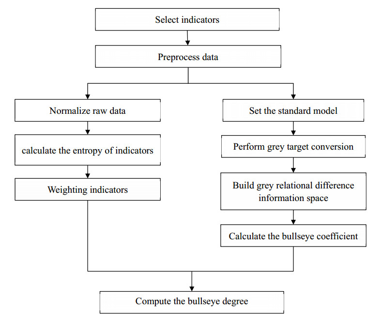
The COVID-19 pandemic has highlighted the importance of the digital economy in restoring economic and social development, creating more jobs and improving people's well-being. To inform policy makers about changes to digital strategies, measuring the digital economy is a prerequisite. This study aimed to compile an index of digital economy at the provincial (municipalities, autonomous regions, collectively referred to as "provinces") level to present an accurate and in-depth depiction of how it has developed in China. Our sample covers 31 provinces in China, over the period 2010–2020. This paper firstly constructs the digital economy index system from the four dimensions of digital users, digital platforms, digital industries and digital innovation, and then adopts a combination of entropy weighting method and grey target theory to measure the digital economy index. This paper study revealed that China's digital economy has been on an upward trend from 2010 to 2019 and has a decline in 2020, and the digital innovation is an important driving force for the growth of the digital economy index. The convergence of China's digital economy is decreasing, indicating that the gap in digital economy development between provinces is increasing. The proposed index in this study can be used as a screening tool, decision making tool, benchmarking tool and guidance of high-quality digital economy development.

| [1] |
Abrell T, Pihlajamaa M, Kanto L (2016) The role of users and customers in digital innovation: Insights from B2B manufacturing firms. Inf Manag 53: 324–335. https://doi.org/10.1016/j.im.2015.12.005 doi: 10.1016/j.im.2015.12.005

|
| [2] | Ali Research Institute, KPMG (2018) 2018 Global Digital Economy Development Index. Available from: http://i.aliresearch.com/img/20180918/20180918153226.pdf. |
| [3] | Atkinson R, Foote C (2021) The 2020 State New Economy Index. Available from: https://www2.itif.org/2020-state-new-economy-index.pdf. |
| [4] |
Baboo S, Nunkoo R, Kock F (2021) Social media attachment: Conceptualization and formative index construction. J Bus Res 139: 437–447. https://doi.org/10.1016/j.jbusres.2021.09.064 doi: 10.1016/j.jbusres.2021.09.064
|
| [5] |
Baker S, Bloom N, Davis S (2016) Measuring Economic Policy Uncertainty. Q J Econ 131: 1593–1636. https://doi.org/10.1093/qje/qjw024 doi: 10.1093/qje/qjw024
|
| [6] | BEA (2018) Defining and Measuring the Digital Economy. Available from: https://www.bea.gov/digital Economy. |
| [7] | BEA (2022) Toward a Digital Economy Satellite Account. Available from: https://www.bea.gov/data/special-topics/digital-economy. |
| [8] |
Beaunoyer E, Dupere S, Guitton MJ (2020) COVID-19 and digital inequalities: Reciprocal impacts and mitigation strategies. Comput Hum Behav 111: 106424. https://doi.org/10.1016/j.chb.2020.106424 doi: 10.1016/j.chb.2020.106424
|
| [9] | CAICT (2017) White Paper on China's Digital Economy Development. Available from: http://www.caict.ac.cn/english/research/whitepapers/. |
| [10] | CAICT (2021) White Paper on China's Digital Economy Development. Available from: http://www.caict.ac.cn/english/research/whitepapers/. |
| [11] | CCID Consulting (2020) Digital Economic Development Index. Available from: http://www.ccidconsulting.com/. |
| [12] | Cornell University (2018) Global Innovation Index 2018: Energizing the World with Innovation. Available from: https://www.wipo.int/publications/en/details.jsp?id=4330. |
| [13] | European Commission (2021) Digital Economy and Society Index. Available from: https://digital-strategy.ec.europa.eu/en/news/digital-economy-and-society-index-2021. |
| [14] |
Golinelli D, Boetto E, Carullo G, et al. (2020) Adoption of Digital Technologies in Health Care During the COVID-19 Pandemic: Systematic Review of Early Scientific Literature. J Med Internet Res 22: e22280. https://doi.org/10.2196/22280 doi: 10.2196/22280
|
| [15] | Government of Australia (2021) Digital economy strategy 2030. Available from: https://apo.org.au/node/312247. |
| [16] |
Hajkowicz S (2006) Multi-attributed environmental index construction. Ecol Econ 57: 122–139. https://doi.org/10.1016/j.ecolecon.2005.03.023 doi: 10.1016/j.ecolecon.2005.03.023
|
| [17] | International Telecommunication Union (2017) Measuring the Information Society Report 2017. Available from: https://www.itu.int/en/ITU-D/Statistics/Pages/publications/mis2017.aspx. |
| [18] |
Lee C, Zhong J (2016) Construction of a responsible investment composite index for renewable energy industry. Renew Sust Energ Rev 51: 288–303. https://doi.org/10.1016/j.rser.2015.05.071 doi: 10.1016/j.rser.2015.05.071
|
| [19] |
Li J, Yu F, Deng G, et al. (2017) Industrial Internet: A Survey on the Enabling Technologies, Applications, and Challenges. IEEE Commun Surv Tutor 19: 1504–1526. https://doi.org/10.1109/COMST.2017.2691349 doi: 10.1109/COMST.2017.2691349
|
| [20] |
Li T, Ma J (2021) Does digital finance benefit the income of rural residents? A case study on China. Quant Financ Econ 4: 664–688. https://doi.org/10.3934/QFE.2021030 doi: 10.3934/QFE.2021030
|
| [21] |
Liao G, Li Z, Wang M, et al. (2022) Measuring China's urban digital finance. Quant Financ Econ 6: 385–404. https://doi.org/10.3934/QFE.2022017 doi: 10.3934/QFE.2022017
|
| [22] | OECD (2014) Measuring the Digital Economy: A New Perspective. http://dx.doi.org/10.1787/9789264221796-en |
| [23] |
Selahattin K, Aykut E, Havvanur F (2021) The effect of COVID-19 pandemic on residential real estate prices: Turkish case. Quant Financ Econ 5: 623–639. https://doi.org/10.3934/QFE.2021028 doi: 10.3934/QFE.2021028
|
| [24] | The 117th Congress (2021) S.1260-United States Innovation and Competition Act of 2021. Available from: https://www.congress.gov/bill/117th-congress/senate-bill/1260. |
| [25] | The World Economic Forum (2021) The Network Readiness Index 2021. Available from: https://networkreadinessindex.org/. |
| [26] | USAID (2021) digital Strategy 2020–2024. Available from: https://www.usaid.gov/usaid-digital-strategy. |
| [27] |
Wang B, Tian J, Cheng L, et al. (2018) Spatial Differentiation of Digital Economy and Its Influencing Factors in China. Sci Geogr Sin 38: 859–868. https://doi.org/10.13249/j.cnki.sgs.2018.06.004 doi: 10.13249/j.cnki.sgs.2018.06.004
|
| [28] |
Whitmore A (2012) A statistical analysis of the construction of the United Nations E-Government Development Index. Gov Inf Q 29: 68–75. https://doi.org/10.1016/j.giq.2011.06.003 doi: 10.1016/j.giq.2011.06.003
|
| [29] | Woetzel J, Seong J, Wang KW, (2017) China's digital economy: A leading global force. Available from: https://www.mckinsey.com/featured-insights/china/chinas-digital-economy-a-leading-global-force. |
| [30] |
Xiang S, Wu W (2019) Research on the Design of China's Digital Economy Satellite Account Framework. Stat Res 36: 3–16. https://doi.org/10.19343/j.cnki.11-1302/c.2019.10.001 doi: 10.19343/j.cnki.11-1302/c.2019.10.001
|
| [31] |
Xu L, Li M, D Q (2017) Dynamic Evaluation Method Based on Grey Target. J Syst Sci Math Sci 37: 112–124. https://doi.org/10.12341/jssms13047 doi: 10.12341/jssms13047
|
| [32] |
Xu X, Zhang M (2020) Research on the Scale Measurement of China's Digital Economy: Based on the Perspective of internet Comparison. China Ind Econ 5: 23–41. https://doi.org/10.19581/j.cnki.ciejournal.2020.05.013 doi: 10.19581/j.cnki.ciejournal.2020.05.013
|
| [33] |
Zhu J, Hipel K (2012) Multiple stages grey target decision making method with incomplete weight based on multi-granularity linguistic label. Inf Sci 212: 15–32. https://doi.org/10.1016/j.ins.2012.05.011 doi: 10.1016/j.ins.2012.05.011
|
| [34] |
Zhu Y, Tian D, Yan F (2020) Effectiveness of Entropy Weight Method in Decision-Making. Math Probl Eng 2020: 3564835. https://doi.org/10.1155/2020/3564835 doi: 10.1155/2020/3564835
|
Figures(1) / Tables(17)

Yanting Xu, Tinghui Li. Measuring digital economy in China[J]. National Accounting Review, 2022, 4(3): 251-272. doi: 10.3934/NAR.2022015


 DownLoad: